graph LR
    Start(( )) --> A1[A1]
    Start --> A2[A2]
    Start --> A3[A3]

    A1 --> BA1["B ∩ A1"]
    A1 --> BcA1["B^c ∩ A1"]

    A2 --> BA2["B ∩ A2"]
    A2 --> BcA2["B^c ∩ A2"]

    A3 --> BA3["B ∩ A3"]
    A3 --> BcA3["B^c ∩ A3"]
MIT 6.041 Probability: Conditioning and Bayes’ Rule
Probability
Conditional Probability
Bayes Rule
Total Probability
MIT 6.041
Conditional probability as belief revision, multiplication and total-probability rules, and Bayes’ rule through die and radar examples from MIT 6.041.
Conditioning
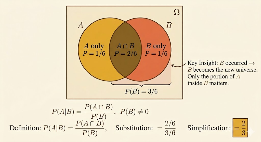
Conditional probability answers the question:
after learning that event \(B\) happened, how should we revise the probability of \(A\)?
The definition is
\[ P(A \mid B) = \frac{P(A \cap B)}{P(B)}, \qquad P(B) > 0. \]
So conditioning does not invent a new probability law. It rescales the old one onto the smaller world where \(B\) is known to have occurred.
Two immediate consequences are:
\[ P(A \cap B) = P(B)\,P(A \mid B) \]
and, symmetrically,
\[ P(A \cap B) = P(A)\,P(B \mid A). \]
Whenever new information arrives, conditional probability is the mathematical way to update our beliefs.
Conditional Additivity
If \(A\) and \(C\) are disjoint, then conditioning preserves additivity:
\[ P(A \cup C \mid B) = P(A \mid B) + P(C \mid B). \]
The reason is simple: inside the conditioned world \(B\), the events \(A \cap B\) and \(C \cap B\) are still disjoint.
Example: Two Rolls of a 4-Sided Die
Roll a 4-sided die twice and write the outcome as \((X,Y)\).
Let
\[ B = \{\min(X,Y)=2\}. \]
The outcomes in \(B\) are:
\[ (2,2), (2,3), (2,4), (3,2), (4,2). \]
So
\[ P(B)=\frac{5}{16}. \]
Now let
\[ M = \max(X,Y). \]
Then:
- \(P(M=1 \mid B)=0\), because \(\min(X,Y)=2\) already forces both rolls to be at least 2
- \(P(M=2 \mid B)=\frac{1}{5}\), because only \((2,2)\) works
You can also compute the second one from the definition:
\[ P(M=2 \mid B) = \frac{P(M=2 \cap B)}{P(B)} = \frac{1/16}{5/16} = \frac{1}{5}. \]
This is a good example of what conditioning does: once we know \(\min(X,Y)=2\), the original uniform \(16\)-point sample space collapses to just \(5\) admissible outcomes.
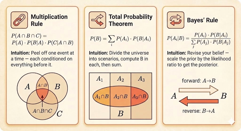
Multiplication Rule
For three events,
\[ P(A \cap B \cap C) = P(A)\,P(B \mid A)\,P(C \mid A \cap B). \]
This comes from applying the two-event multiplication rule twice:
\[ P(A \cap B \cap C) = P((A \cap B)\cap C) = P(A \cap B)\,P(C \mid A \cap B) = P(A)\,P(B \mid A)\,P(C \mid A \cap B). \]
The general pattern is:
\[ P(A_1 \cap A_2 \cap \cdots \cap A_n) = P(A_1)P(A_2 \mid A_1)\cdots P(A_n \mid A_1 \cap \cdots \cap A_{n-1}). \]
Total Probability
Suppose \(A_1,\dots,A_n\) form a partition of the sample space:
- they are disjoint
- their union is the whole sample space
Then any event \(B\) can be decomposed as
\[ B = (B \cap A_1)\cup \cdots \cup (B \cap A_n), \]
with disjoint pieces. Therefore
\[ P(B)=\sum_{i=1}^n P(B \cap A_i) = \sum_{i=1}^n P(A_i)\,P(B \mid A_i). \]
This is the total probability formula.
Conceptually, this says:
- first choose which case \(A_i\) happened
- then ask how likely \(B\) is inside that case
Bayes’ Rule
Now reverse the conditioning direction.
If \(A_1,\dots,A_n\) form a partition and \(P(B)>0\), then
\[ P(A_i \mid B) = \frac{P(A_i \cap B)}{P(B)} = \frac{P(A_i)\,P(B \mid A_i)}{\sum_j P(A_j)\,P(B \mid A_j)}. \]
This is Bayes’ rule.
It has a clean interpretation:
- \(P(A_i)\) is the prior belief
- \(P(B \mid A_i)\) is the likelihood
- \(P(A_i \mid B)\) is the posterior belief after seeing evidence \(B\)
So Bayes’ rule is fundamentally a rule for belief revision.
Radar Example
Let:
- \(A\) = “a plane is present”
- \(B\) = “the radar reports a signal”
Suppose:
\[ P(A)=0.05, \qquad P(A^c)=0.95, \]
\[ P(B \mid A)=0.99, \qquad P(B \mid A^c)=0.10. \]
Step 1: Joint Probability
\[ P(A \cap B)=P(A)\,P(B \mid A)=0.05 \cdot 0.99 = 0.0495. \]
Step 2: Total Probability of a Signal
Using total probability,
\[ P(B)=P(A)P(B \mid A)+P(A^c)P(B \mid A^c) \]
so
\[ P(B)=0.05\cdot 0.99 + 0.95\cdot 0.10 = 0.1445. \]
Step 3: Posterior Probability of a Plane
Now apply Bayes’ rule:
\[ P(A \mid B)=\frac{P(A \cap B)}{P(B)} = \frac{0.0495}{0.1445} \approx 0.343. \]
So even after a positive radar signal, the probability that a plane is actually present is only about \(34.3\%\).
This is the classic lesson:
- the radar is very sensitive
- but false alarms are not rare
- and planes are rare to begin with
Rare priors can dominate strong-looking evidence.
Takeaways
- conditioning means revising probabilities after learning new information
- the multiplication rule converts conditional probabilities into joint probabilities
- the total probability formula sums over a partition of mutually exclusive cases
- Bayes’ rule reverses conditioning and turns priors into posteriors
- in applications, the base rate matters as much as the sensor accuracy