MIT 6.041 Probability: Discrete Random Variables I
Random Variables
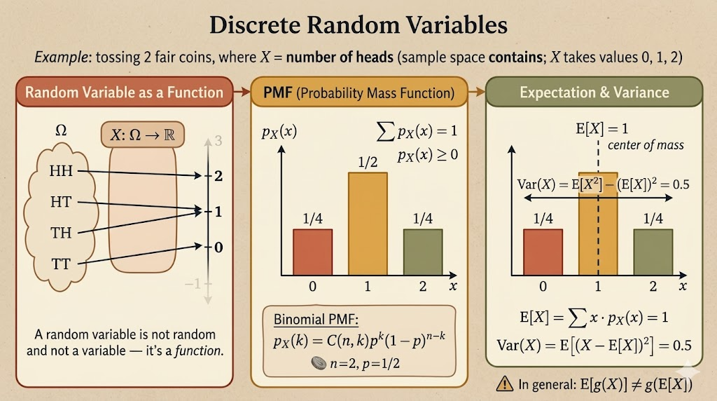
A random variable is an assignment of a numerical value to every possible outcome of an experiment.
Mathematically, if the sample space is \(\Omega\), then a random variable is a function
\[ X:\Omega \to \mathbb{R}. \]
This definition is worth taking literally:
- it is not random
- it is not a variable in the algebraic sense
- it is a function from outcomes to numbers
- its possible values can be discrete or continuous
The randomness comes from the outcome \(\omega \in \Omega\). Once \(\omega\) is known, \(X(\omega)\) is just a number.
Probability Mass Function
For a discrete random variable, the probability mass function (PMF) is
\[ p_X(x) = P(X=x). \]
Equivalently,
\[ p_X(x) = P(\{\omega \in \Omega : X(\omega)=x\}). \]
The PMF must satisfy two basic properties:
\[ p_X(x) \ge 0 \]
and
\[ \sum_x p_X(x) = 1. \]
So the PMF transfers probability from the original sample space onto the numerical values that \(X\) can take.
Example: First Head
Flip a biased coin repeatedly until the first head appears. Suppose
\[ P(H)=p,\qquad P(T)=1-p. \]
Let \(X\) be the number of tosses until the first head.
Then:
- \(X=1\) for outcome \(H\)
- \(X=2\) for outcome \(TH\)
- \(X=k\) for outcome \(\underbrace{TT\cdots T}_{k-1}H\)
Therefore the PMF is
\[ p_X(k) = P(X=k) = (1-p)^{k-1}p, \qquad k=1,2,\dots. \]
This is the geometric distribution. The value \(k\) records how long we waited before the first success.
Example: Two Four-Sided Dice
Roll two independent fair four-sided dice. Let \(F\) be the first roll and \(S\) be the second roll, so
\[ \Omega = \{(F,S): F,S \in \{1,2,3,4\}\}. \]
There are \(16\) equally likely outcomes.
Define
\[ X = \min(F,S). \]
For example, \(X=2\) when the smaller of the two rolls is exactly \(2\). The outcomes are:
\[ (2,2), (2,3), (2,4), (3,2), (4,2). \]
So
\[ p_X(2) = \frac{5}{16}. \]
One way to see the full PMF is to count the outcomes where the minimum is each possible value:
| \(x\) | outcomes with \(\min(F,S)=x\) | \(p_X(x)\) |
|---|---|---|
| 1 | 7 | \(7/16\) |
| 2 | 5 | \(5/16\) |
| 3 | 3 | \(3/16\) |
| 4 | 1 | \(1/16\) |
The probabilities add to one:
\[ \frac{7+5+3+1}{16}=1. \]
Example: Number of Heads
Flip a coin \(n\) times, and let \(X\) be the number of heads.
For \(n=4\), the probability of exactly two heads is
\[ \begin{aligned} p_X(2) &= P(HHTT) + P(HTHT) + P(HTTH) \\ &\quad + P(THHT) + P(THTH) + P(TTHH) \\ &= 6p^2(1-p)^2 \\ &= \binom{4}{2}p^2(1-p)^2. \end{aligned} \]
In general,
\[ p_X(k) = \binom{n}{k}p^k(1-p)^{n-k}, \qquad k=0,1,\dots,n. \]
This is the binomial distribution. The binomial coefficient counts which \(k\) tosses are heads, while \(p^k(1-p)^{n-k}\) gives the probability of any one such sequence.
Expectation
The expected value of a discrete random variable is its probability-weighted average:
\[ E[X] = \sum_x x\,p_X(x). \]
For example, suppose a payoff \(X\) has PMF
\[ P(X=1)=\frac{1}{6},\qquad P(X=2)=\frac{1}{2},\qquad P(X=4)=\frac{1}{3}. \]
Then
\[ \begin{aligned} E[X] &= 1\cdot \frac{1}{6} + 2\cdot \frac{1}{2} + 4\cdot \frac{1}{3} \\ &= \frac{1}{6}+1+\frac{4}{3} \\ &= 2.5. \end{aligned} \]
The expectation is not necessarily a value that the random variable can actually take. In this example, \(2.5\) is the long-run average payoff, not one possible payoff.
Functions of Random Variables
Suppose
\[ Y = g(X). \]
One way to find \(E[Y]\) is to first derive the PMF of \(Y\) and then compute
\[ E[Y] = \sum_y y\,p_Y(y). \]
But there is an easier shortcut:
\[ E[g(X)] = \sum_x g(x)\,p_X(x). \]
This says we can average the transformed values \(g(x)\) using the original PMF of \(X\).
In general,
\[ E[g(X)] \ne g(E[X]). \]
For example, usually
\[ E[X^2] \ne (E[X])^2. \]
Linearity Properties
For constants \(\alpha\) and \(\beta\),
\[ E[\alpha] = \alpha, \]
\[ E[\alpha X] = \alpha E[X], \]
and
\[ E[\alpha X + \beta] = \alpha E[X] + \beta. \]
These properties are often the fastest way to compute expectations without expanding every outcome.
Variance
Expectation gives the center of a distribution. Variance measures spread around that center.
The second moment is
\[ E[X^2] = \sum_x x^2 p_X(x). \]
The variance is
\[ \operatorname{var}(X) = E[(X-E[X])^2]. \]
Expanding this expression gives the useful computational formula:
\[ \begin{aligned} \operatorname{var}(X) &= \sum_x (x-E[X])^2p_X(x) \\ &= E[X^2] - (E[X])^2. \end{aligned} \]
Two basic properties are:
\[ \operatorname{var}(X) \ge 0 \]
and
\[ \operatorname{var}(\alpha X+\beta) = \alpha^2 \operatorname{var}(X). \]
Adding a constant shifts the distribution but does not change its spread. Multiplying by \(\alpha\) scales deviations by \(\alpha\), so variance scales by \(\alpha^2\).
Summary
- A random variable is a function from outcomes to real numbers.
- A PMF assigns probability to the possible values of a discrete random variable.
- Common discrete distributions include the geometric distribution and binomial distribution.
- Expectation is a probability-weighted average.
- For functions of a random variable, \(E[g(X)]\) can be computed directly from the PMF of \(X\).
- Variance measures spread and satisfies \(\operatorname{var}(X)=E[X^2]-(E[X])^2\).