MIT 6.041 Probability: Discrete Random Variables II
Conditional PMF
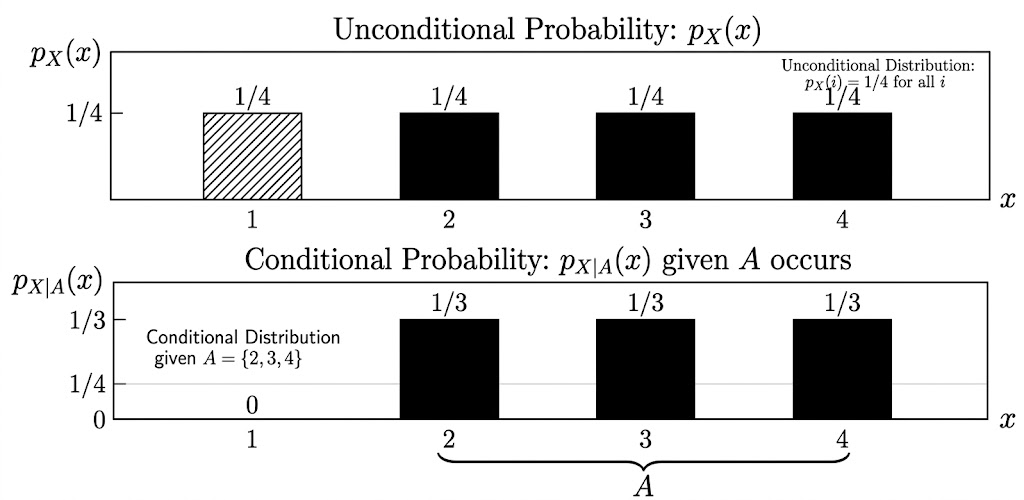
A conditional PMF is the distribution of a random variable after we learn that an event occurred.
If \(A\) is an event with \(P(A)>0\), then
\[ p_{X|A}(x) = P(X=x \mid A). \]
This is still a valid PMF over the possible values of \(X\):
\[ p_{X|A}(x) \ge 0, \qquad \sum_x p_{X|A}(x)=1. \]
The only difference is that probability is now normalized inside the world where \(A\) has happened.
Conditional Expectation
Once we have a conditional PMF, we can compute a conditional expectation:
\[ E[X \mid A] = \sum_x x\,p_{X|A}(x). \]
So conditional expectation is the average value of \(X\) after restricting attention to outcomes in \(A\).
For example, suppose \(X\) takes values \(1,2,3,4\) and we condition on
\[ A=\{X \ge 2\}. \]
If the conditional PMF is
\[ p_{X|A}(x)=\frac{1}{3}, \qquad x=2,3,4, \]
then
\[ E[X \mid A] = \frac{1}{3}\cdot 2 + \frac{1}{3}\cdot 3 + \frac{1}{3}\cdot 4 =3. \]
The point is that conditioning changes the distribution first. Expectation is then computed with respect to that new distribution.
Geometric PMF
Let \(X\) be the number of independent coin tosses required until the first head appears.
If
\[ P(H)=p, \qquad P(T)=1-p, \]
then
\[ p_X(k) = P(X=k) = (1-p)^{k-1}p, \qquad k=1,2,3,\dots. \]
This is the geometric distribution. The event \(X=k\) means:
- the first \(k-1\) tosses are tails
- the \(k\)th toss is the first head
The expectation is
\[ E[X] = \sum_{k=1}^{\infty} k(1-p)^{k-1}p. \]
The final result is
\[ E[X]=\frac{1}{p}. \]
So if a head has probability \(p=1/3\), the expected waiting time until the first head is \(3\) tosses.
Memoryless Property
The geometric distribution has a special property: after failures, the future looks like a fresh start.
For example, suppose we know the first two tosses were tails. This is the event
\[ X>2. \]
The distribution of the additional waiting time is the same as the original distribution:
\[ P(X-2=k \mid X>2) = P(X=k). \]
More generally,
\[ P(X-n=k \mid X>n) = P(X=k), \qquad k=1,2,\dots. \]
Equivalently,
\[ P(X>n+k \mid X>n) = P(X>k). \]
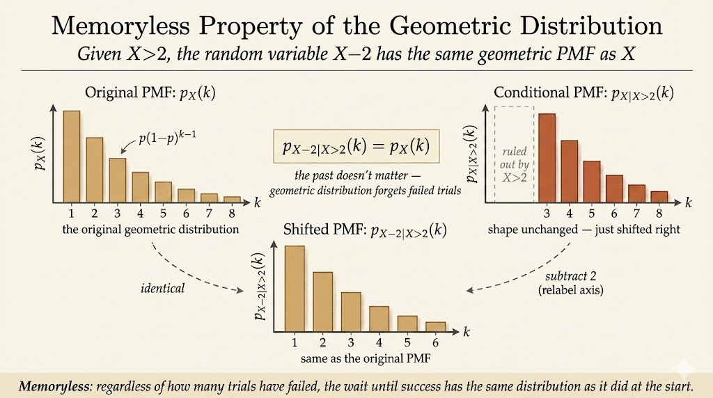
This is why the geometric distribution is called memoryless. The coin does not remember previous tails. If the first \(8\) tosses were tails, the expected number of additional tosses is still \(E[X]\).
Therefore the total expected number of tosses, given that the first \(8\) tosses failed, is
\[ 8 + E[X]. \]
Total Expectation
The total probability theorem decomposes an event by cases:
\[ P(B) = P(A_1)P(B \mid A_1) + \cdots + P(A_n)P(B \mid A_n), \]
where \(A_1,\dots,A_n\) form a partition of the sample space.
The same idea applies to PMFs:
\[ p_X(x) = P(A_1)p_{X|A_1}(x) + \cdots + P(A_n)p_{X|A_n}(x). \]
Taking the weighted average over \(x\) gives the total expectation theorem:
\[ E[X] = P(A_1)E[X \mid A_1] + \cdots + P(A_n)E[X \mid A_n]. \]
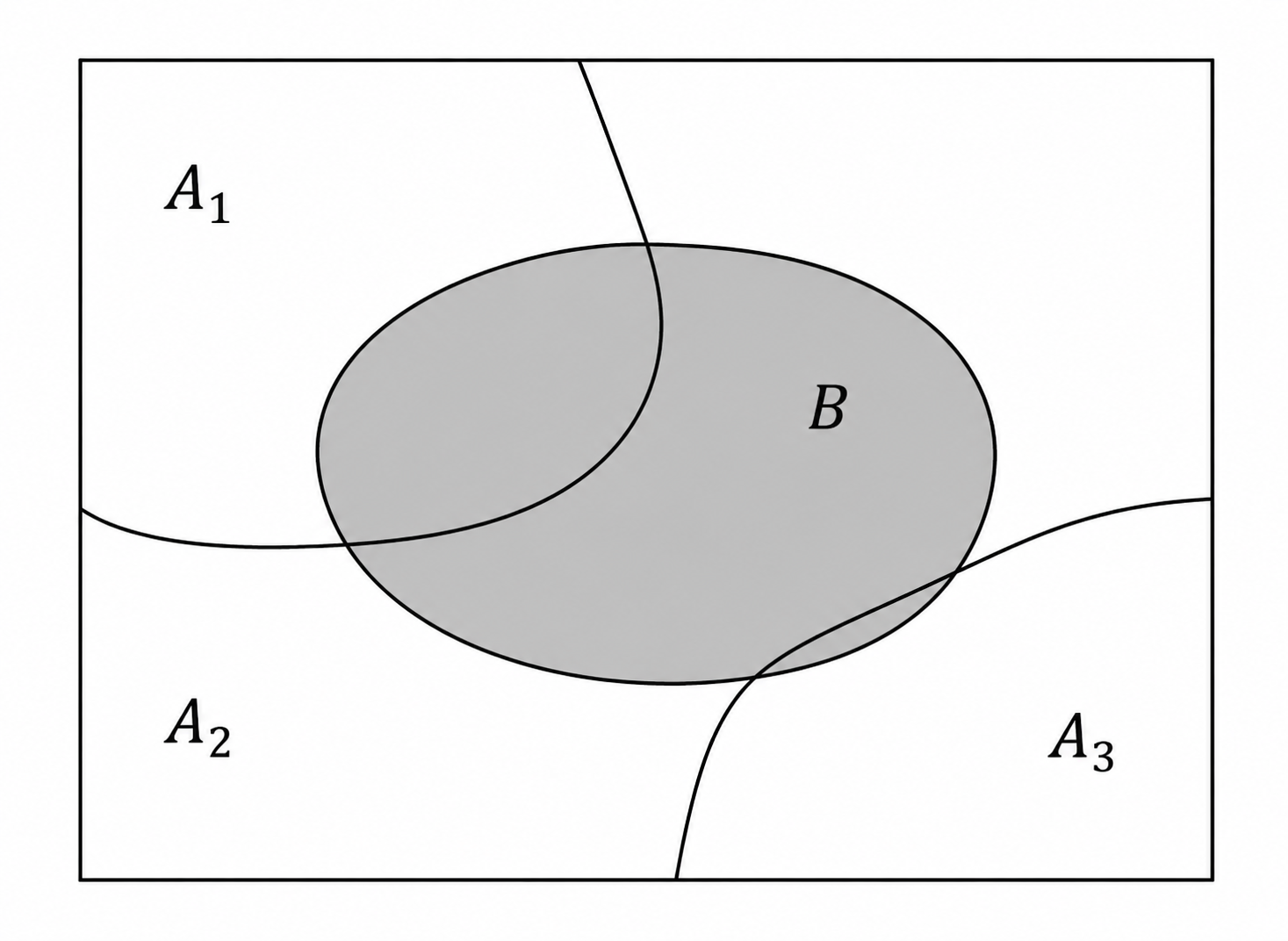
The theorem says that we can compute an expectation by splitting the world into cases, computing the conditional average in each case, and weighting by the probability of each case.
Geometric Expectation by Conditioning
The geometric distribution gives a clean example of total expectation.
Let \(X\) be the first time we see a head. Split the sample space into two cases:
\[ A_1=\{X=1\}, \qquad A_2=\{X>1\}. \]
Then
\[ E[X] = P(X=1)E[X \mid X=1] + P(X>1)E[X \mid X>1]. \]
The pieces are:
\[ P(X=1)=p, \qquad E[X \mid X=1]=1, \]
and
\[ P(X>1)=1-p. \]
If the first toss is a tail, then one toss has already happened, and by memorylessness the expected additional waiting time is still \(E[X]\):
\[ E[X \mid X>1] = 1+E[X]. \]
Therefore
\[ E[X] = p\cdot 1 + (1-p)(1+E[X]). \]
Solving,
\[ \begin{aligned} E[X] &=p+(1-p)+(1-p)E[X] \\ &=1+(1-p)E[X], \end{aligned} \]
so
\[ pE[X]=1, \qquad E[X]=\frac{1}{p}. \]
This derivation shows why the result is natural: each failed toss resets the probabilistic situation, but it still adds one unit of time already spent.
Joint PMFs
For two discrete random variables \(X\) and \(Y\), the joint PMF is
\[ p_{X,Y}(x,y) = P(X=x,\;Y=y). \]
It describes the probability of every pair of values.
A joint PMF must satisfy
\[ p_{X,Y}(x,y)\ge 0 \]
and
\[ \sum_x \sum_y p_{X,Y}(x,y)=1. \]
For example:
| \(Y\backslash X\) | \(x=1\) | \(x=2\) | \(x=3\) | \(x=4\) |
|---|---|---|---|---|
| \(y=4\) | \(1/20\) | \(2/20\) | \(2/20\) | \(0\) |
| \(y=3\) | \(2/20\) | \(4/20\) | \(1/20\) | \(2/20\) |
| \(y=2\) | \(0\) | \(1/20\) | \(3/20\) | \(1/20\) |
| \(y=1\) | \(0\) | \(1/20\) | \(0\) | \(0\) |
From the joint PMF, we can recover the marginal PMFs by summing out the other variable:
\[ p_X(x) = \sum_y p_{X,Y}(x,y), \]
and
\[ p_Y(y) = \sum_x p_{X,Y}(x,y). \]
We can also form conditional PMFs:
\[ p_{X|Y}(x \mid y) = P(X=x \mid Y=y) = \frac{p_{X,Y}(x,y)}{p_Y(y)}, \]
as long as \(p_Y(y)>0\).
For each fixed \(y\),
\[ \sum_x p_{X|Y}(x \mid y)=1. \]
Takeaways
- Conditional PMFs are ordinary PMFs after restricting to an event.
- Conditional expectation is expectation computed under that conditional PMF.
- The geometric distribution is memoryless: after failures, the future waiting time has the same distribution as at the start.
- Total expectation decomposes an average into case-by-case conditional averages.
- A joint PMF describes two random variables together; marginal and conditional PMFs come from summing or normalizing it.
Source: MIT 6.041 Probabilistic Systems Analysis and Applied Probability, Lecture 6.