MIT 6.041 Probability: Discrete Random Variables III
This lecture extends discrete random variables from one or two variables to several variables.
The main ideas are:
- joint PMFs can be marginalized to get individual PMFs
- multiplication rules factor joint probabilities into conditional probabilities
- expectation is linear even without independence
- variance adds only when covariance terms vanish, such as under independence
- indicator variables make many counting expectations much easier
Three Random Variables
For three discrete random variables \(X,Y,Z\), the joint PMF is
\[ p_{X,Y,Z}(x,y,z) = P(X=x,Y=y,Z=z). \]
We can recover the marginal PMF of \(X\) by summing over the other variables:
\[ p_X(x) = \sum_y \sum_z p_{X,Y,Z}(x,y,z). \]
The same idea works for any subset of variables. Marginalization means summing out the variables we no longer want to track.
Multiplication Rule
For three events \(A,B,C\), the multiplication rule is
\[ P(A \cap B \cap C) = P(A)P(B \mid A)P(C \mid A \cap B). \]
For random variables, this becomes
\[ p_{X,Y,Z}(x,y,z) = p_X(x) p_{Y\mid X}(y\mid x) p_{Z\mid X,Y}(z\mid x,y). \]
This is useful because a complicated joint probability can be built as a sequence of conditional probabilities.
If \(X,Y,Z\) are independent, the factorization simplifies to
\[ p_{X,Y,Z}(x,y,z) = p_X(x)p_Y(y)p_Z(z). \]
Independence means that learning one variable does not change the distribution of the others. For example, if \(X\) and \(Y\) are independent, then
\[ p_{X\mid Y}(x\mid y) = p_X(x). \]
If \(X,Y,Z\) are mutually independent, then
\[ p_{X\mid Y,Z}(x\mid y,z) = p_X(x). \]
Knowing both \(Y\) and \(Z\) still gives no information about \(X\).
Expectations of Functions
For two discrete random variables, the expectation of a function \(g(X,Y)\) is computed by summing over all pairs:
\[ E[g(X,Y)] = \sum_x \sum_y g(x,y)p_{X,Y}(x,y). \]
In general,
\[ E[g(X,Y)] \ne g(E[X],E[Y]). \]
Expectation applies to the function values over all outcomes, not just to the function evaluated at the average inputs.
Linearity of Expectation
The most important expectation rule is linearity:
\[ E[X+Y+Z] = E[X]+E[Y]+E[Z]. \]
This is true whether or not the random variables are independent.
Independence is not needed because the joint PMF marginalizes correctly when summing:
\[ E[X+Y] = \sum_x\sum_y (x+y)p_{X,Y}(x,y) = E[X]+E[Y]. \]
Product of Independent Variables
If \(X\) and \(Y\) are independent, then
\[ E[XY] = E[X]E[Y]. \]
More generally, if \(X\) and \(Y\) are independent, then any functions of them are also independent:
\[ E[g(X)h(Y)] = E[g(X)]E[h(Y)]. \]
This product rule does require independence. Linearity of expectation does not.
Variance of Sums
Variance is different from expectation. It is not always additive.
In general,
\[ \operatorname{Var}(X+Y) = \operatorname{Var}(X) + \operatorname{Var}(Y) + 2\operatorname{Cov}(X,Y). \]
If \(X\) and \(Y\) are independent, then \(\operatorname{Cov}(X,Y)=0\), so
\[ \operatorname{Var}(X+Y) = \operatorname{Var}(X) + \operatorname{Var}(Y). \]
For example, if \(X\) and \(Y\) are independent, then
\[ \operatorname{Var}(X-3Y) = \operatorname{Var}(X) + 9\operatorname{Var}(Y). \]
The coefficient is squared because variance measures squared deviation.
Binomial Expectation and Variance
Let
\[ X \sim \operatorname{Binomial}(n,p). \]
The PMF is
\[ p_X(k) = \binom{n}{k}p^k(1-p)^{n-k}, \qquad k=0,1,\dots,n. \]
Directly computing the expectation from
\[ E[X] = \sum_{k=0}^{n} k\binom{n}{k}p^k(1-p)^{n-k} \]
is possible, but there is a much cleaner method.
Write \(X\) as a sum of indicator variables:
\[ X=X_1+\cdots+X_n, \]
where
\[ X_i = \begin{cases} 1, & \text{trial } i \text{ succeeds},\\ 0, & \text{trial } i \text{ fails}. \end{cases} \]
Each \(X_i\) is a Bernoulli random variable with
\[ E[X_i]=p. \]
By linearity of expectation,
\[ E[X] = \sum_{i=1}^n E[X_i] = np. \]
For one Bernoulli trial,
\[ \operatorname{Var}(X_i) = p(1-p). \]
Because the trials are independent, the variances add:
\[ \operatorname{Var}(X) = \sum_{i=1}^n \operatorname{Var}(X_i) = np(1-p). \]
The indicator-variable viewpoint avoids tedious algebra and reveals the structure of the binomial distribution.
The Hat Problem
Suppose \(n\) people check their hats at a party. The attendant randomly permutes the hats before returning them.
Let \(X\) be the number of people who get their own hat back.
Expected Number of Matches
Define the indicator variable
\[ X_i = \begin{cases} 1, & \text{person } i \text{ gets their own hat},\\ 0, & \text{otherwise}. \end{cases} \]
Then
\[ X=X_1+\cdots+X_n. \]
For any person \(i\),
\[ P(X_i=1)=\frac{1}{n}, \]
so
\[ E[X_i]=\frac{1}{n}. \]
By linearity of expectation,
\[ E[X] = \sum_{i=1}^n E[X_i] = n\cdot \frac{1}{n} = 1. \]
So no matter how many people attend, the expected number of people who get their own hat back is \(1\).
Variance of the Number of Matches
For \(n \ge 2\),
\[ \operatorname{Var}(X) = E[X^2]-(E[X])^2 = E[X^2]-1. \]
Expand \(X^2\):
\[ X^2 = \left(\sum_{i=1}^n X_i\right)^2 = \sum_{i=1}^n X_i^2 + \sum_{i\ne j}X_iX_j. \]
Since \(X_i\) is an indicator variable,
\[ X_i^2=X_i. \]
Therefore
\[ \sum_{i=1}^n E[X_i^2] = \sum_{i=1}^n E[X_i] = 1. \]
For the cross terms, \(X_iX_j=1\) only if both person \(i\) and person \(j\) get their own hats. For \(i\ne j\),
\[ E[X_iX_j] = P(X_i=1,X_j=1) = \frac{1}{n}\cdot\frac{1}{n-1}. \]
There are \(n(n-1)\) ordered cross terms, so
\[ \sum_{i\ne j}E[X_iX_j] = n(n-1)\cdot \frac{1}{n(n-1)} = 1. \]
Thus
\[ E[X^2]=1+1=2, \]
and
\[ \operatorname{Var}(X) = 2-1^2 = 1. \]
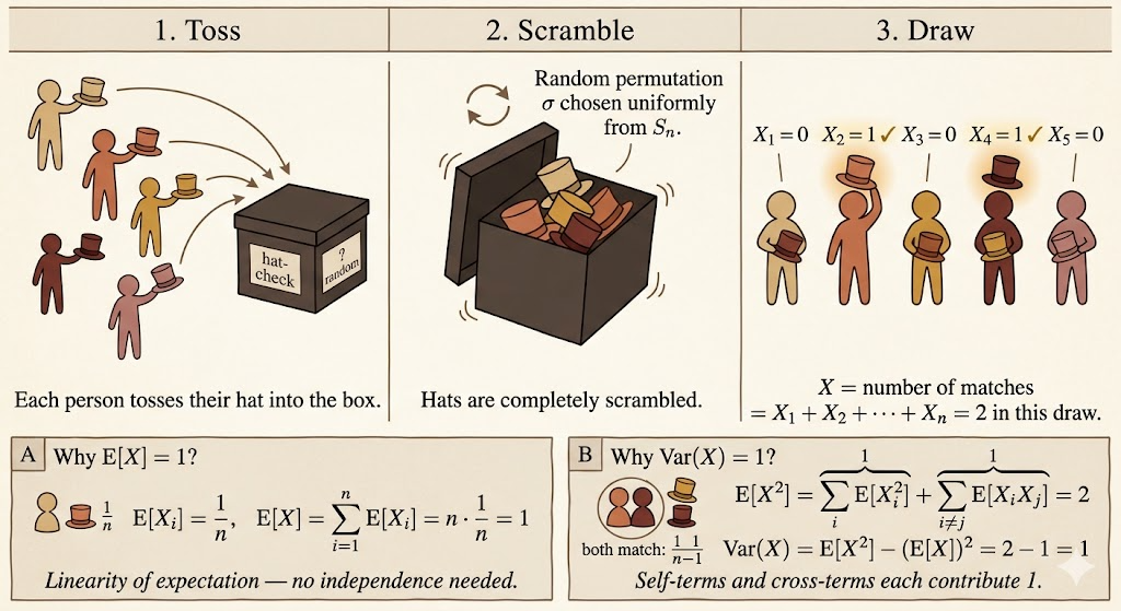
The important lesson is that the indicators are not independent, but linearity of expectation still gives the mean immediately. For variance, we must handle the cross terms.
Summary
- Joint PMFs for multiple random variables can be marginalized by summing out variables.
- The multiplication rule factors joint probabilities into conditional probabilities.
- Linearity of expectation does not require independence.
- Products of expectations usually require independence.
- Variance of a sum includes covariance terms unless the variables are independent.
- Indicator variables make binomial and matching problems much easier.