MIT 6.041 Probability: Continuous Bayes’ Rule and Derived Distributions
This lecture connects two recurring probability themes:
- how Bayes’ rule works when densities replace probabilities
- how to derive the distribution of a new random variable from an old one
The main shift is conceptual. In continuous models, point probabilities are zero, so inference and transformation are expressed through PDFs, CDFs, and integrals.
The Bayes Variation
The Bayes setup can be viewed as a noisy measurement process.
There is an unknown quantity \(X\), a device or channel that produces an observation, and an observed output \(Y\).
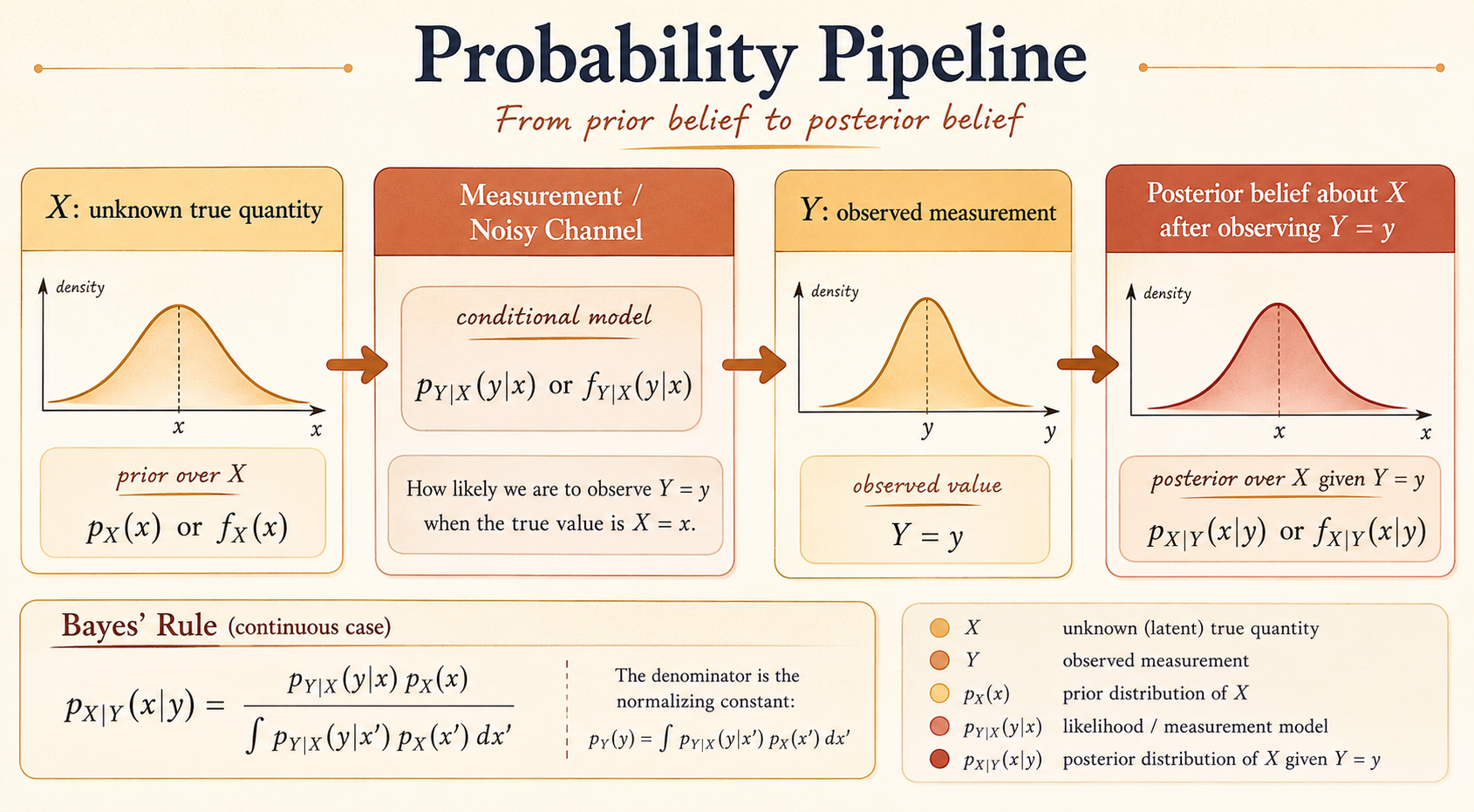
Input: \(X\)
\(X\) is the true underlying signal or quantity we want to infer. Examples include the actual temperature, a transmitted signal, or the location of an aircraft.
- \(p_X(x)\): prior PMF for \(X\) when \(X\) is discrete.
- \(f_X(x)\): prior PDF for \(X\) when \(X\) is continuous.
Measurement Model
The measurement model describes the randomness or noise in the observation process. It tells us how likely each output is for a given input.
- \(p_{Y|X}(y|x)\): conditional PMF in the discrete case.
- \(f_{Y|X}(y|x)\): conditional PDF in the continuous case.
Output: \(Y\)
\(Y\) is the actual measurement or observation. Once we observe \(Y=y\), Bayes’ rule updates our belief about the hidden input \(X\).
Examples
Discrete Example: Radar
The radar example is a discrete Bayes model.
- \(X=1\): an airplane is present.
- \(X=0\): no airplane is present.
- \(Y=1\): something registers on the radar screen.
- \(Y=0\): nothing registers on the radar screen.
The conditional PMF \(p_{Y|X}(y|x)\) captures false alarms and missed detections:
- \(p_{Y|X}(1|0)\): false alarm probability.
- \(p_{Y|X}(0|1)\): missed detection probability.
After observing \(Y=y\), the posterior \(p_{X|Y}(x|y)\) tells us how likely it is that an airplane is actually present.
Continuous Example: Signal plus Noise
The signal example is a continuous Bayes model.
- \(X\): the true underlying signal.
- \(f_X(x)\): prior density over possible signal values.
- \(Y\): the noisy version of \(X\) that we observe.
- \(f_{Y|X}(y|x)\): the noise model.
After observing \(Y=y\), continuous Bayes’ rule gives \(f_{X|Y}(x|y)\), the posterior density over the true signal.
Bayes’ Rule
For discrete random variables:
\[ p_{X|Y}(x|y) = \frac{p_X(x)p_{Y|X}(y|x)}{p_Y(y)} \]
where
\[ p_Y(y) = \sum_x p_X(x)p_{Y|X}(y|x). \]
For continuous random variables:
\[ f_{X|Y}(x|y) = \frac{f_X(x)f_{Y|X}(y|x)}{f_Y(y)} \]
where
\[ f_Y(y) = \int_{-\infty}^{\infty} f_X(x)f_{Y|X}(y|x)\,dx. \]
The structure is the same:
\[ \text{posterior} = \frac{\text{prior}\times \text{likelihood}}{\text{evidence}}. \]
The denominator normalizes the posterior so it integrates or sums to 1.
Mixed Cases in Bayesian Inference
Bayes’ rule can mix discrete and continuous random variables. The main rule is to match the type of the variable being inferred.
- If \(X\) is discrete, the posterior over \(X\) is a PMF.
- If \(X\) is continuous, the posterior over \(X\) is a PDF.
- The denominator is always the marginal distribution of the observation \(Y\).
Discrete \(X\), Continuous \(Y\)
Here \(X\) takes discrete values, but the observation \(Y\) is continuous.
The posterior over \(X\) is a PMF:
\[ p_{X|Y}(x|y) = \frac{p_X(x)f_{Y|X}(y|x)}{f_Y(y)}. \]
The marginal density of \(Y\) is
\[ f_Y(y) = \sum_x p_X(x)f_{Y|X}(y|x). \]
Example: a discrete signal is sent through a continuous noisy channel. After observing \(Y=y\), the posterior \(p_{X|Y}(x|y)\) tells us which discrete signal value was most likely sent.
Continuous \(X\), Discrete \(Y\)
Here \(X\) is continuous, but the observation \(Y\) is discrete.
The posterior over \(X\) is a PDF:
\[ f_{X|Y}(x|y) = \frac{f_X(x)p_{Y|X}(y|x)}{p_Y(y)}. \]
The marginal PMF of \(Y\) is
\[ p_Y(y) = \int_{-\infty}^{\infty} f_X(x)p_{Y|X}(y|x)\,dx. \]
Example: a continuous physical quantity affects a discrete measurement or decision. After observing \(Y=y\), the posterior \(f_{X|Y}(x|y)\) gives a density over possible values of the continuous signal.
Derived Distributions
A derived distribution is the distribution of a new random variable defined as a function of one or more existing random variables.
If \(Y=g(X)\) and the distribution of \(X\) is known, the distribution of \(Y\) is derived from the distribution of \(X\).
Discrete Case
For a discrete random variable \(X\), collect all input values that map to the same output value \(y\):
\[ p_Y(y) = P(g(X)=y) = \sum_{x:g(x)=y} p_X(x). \]
Continuous Case
For a continuous random variable \(X\), it is often easiest to start from the CDF:
\[ F_Y(y) = P(Y\le y) = P(g(X)\le y). \]
Then translate the event back into the \(X\) domain and integrate the known density \(f_X(x)\) over the corresponding region.
Once \(F_Y(y)\) is known, differentiate:
\[ f_Y(y) = \frac{d}{dy}F_Y(y). \]
Example: Derived Distribution of Travel Time
Suppose the distance is fixed, but the speed is random.
- Distance: \(D=200\) miles.
- Speed: \(V\sim \operatorname{Uniform}(30,60)\) mph.
- Time: \(T=200/V\) hours.
The PDF of the speed is
\[ f_V(v) = \frac{1}{30}, \qquad 30\le v\le 60. \]
The goal is to find \(f_T(t)\).
Step 1: Determine the Range of \(T\)
The fastest speed gives the shortest time:
\[ t_{\min} = \frac{200}{60} = \frac{10}{3}. \]
The slowest speed gives the longest time:
\[ t_{\max} = \frac{200}{30} = \frac{20}{3}. \]
So
\[ \frac{10}{3} \le T \le \frac{20}{3}. \]
Step 2: Find the CDF
Start from the definition:
\[ F_T(t) = P(T\le t). \]
Substitute \(T=200/V\):
\[ F_T(t) = P\left(\frac{200}{V}\le t\right). \]
Since \(V>0\) and \(t>0\):
\[ F_T(t) = P\left(V\ge \frac{200}{t}\right). \]
For \(\frac{10}{3}\le t\le \frac{20}{3}\):
\[ F_T(t) = \int_{200/t}^{60} \frac{1}{30}\,dv = \frac{1}{30} \left(60-\frac{200}{t}\right) = 2-\frac{20}{3t}. \]
Including the full support:
\[ F_T(t) = \begin{cases} 0, & t<\frac{10}{3}, \\ 2-\frac{20}{3t}, & \frac{10}{3}\le t\le \frac{20}{3}, \\ 1, & t>\frac{20}{3}. \end{cases} \]
Step 3: Differentiate to Get the PDF
For \(\frac{10}{3}\le t\le \frac{20}{3}\):
\[ f_T(t) = \frac{d}{dt} \left(2-\frac{20}{3t}\right) = \frac{20}{3t^2}. \]
Therefore,
\[ f_T(t) = \begin{cases} \frac{20}{3t^2}, & \frac{10}{3}\le t\le \frac{20}{3}, \\ 0, & \text{otherwise}. \end{cases} \]
The density is larger near smaller times because small travel times correspond to higher speeds. The transformation \(T=200/V\) reverses order: larger \(V\) means smaller \(T\).
PDF of \(Y=aX+b\)
A linear transformation rescales and shifts a continuous random variable.
Let
\[ Y=aX+b, \qquad a\ne 0. \]
The inverse transformation is
\[ X = \frac{Y-b}{a}. \]
The PDF of \(Y\) is
\[ f_Y(y) = \frac{1}{|a|} f_X\left(\frac{y-b}{a}\right). \]
Interpretation:
- \(\frac{y-b}{a}\) maps the value \(y\) back to the corresponding value of \(X\).
- \(\frac{1}{|a|}\) rescales the height so the total area under the PDF remains 1.
- The absolute value is needed because densities are nonnegative even when the transformation reverses direction.
Geometric Intuition
A linear transformation has two effects.
- Multiplying by \(a\) stretches or compresses the horizontal axis. The PDF height changes by the reciprocal factor \(1/|a|\).
- Adding \(b\) shifts the distribution left or right without changing its shape.
For example, if \(Y=2X+5\):
\[ f_Y(y) = \frac{1}{2} f_X\left(\frac{y-5}{2}\right). \]
![]()
The center moves from 0 to 5, the width doubles, and the peak density is halved.
Deriving the CDF for \(a>0\)
For positive \(a\):
\[ F_Y(y) = P(Y\le y) = P(aX+b\le y). \]
Because \(a>0\), dividing by \(a\) does not flip the inequality:
\[ P(aX+b\le y) = P\left(X\le \frac{y-b}{a}\right). \]
Therefore,
\[ F_Y(y) = F_X\left(\frac{y-b}{a}\right). \]
Differentiate with respect to \(y\):
\[ f_Y(y) = \frac{d}{dy} F_X\left(\frac{y-b}{a}\right) = \frac{1}{a} f_X\left(\frac{y-b}{a}\right). \]
For negative \(a\), the inequality reverses in the CDF step, but the final density is handled by the absolute value:
\[ f_Y(y) = \frac{1}{|a|} f_X\left(\frac{y-b}{a}\right). \]
Normal Distribution Takeaway
If
\[ X\sim \mathcal{N}(\mu,\sigma^2), \]
then
\[ Y=aX+b \sim \mathcal{N}(a\mu+b,\ a^2\sigma^2). \]
A linear transformation changes the mean and variance, but it preserves the normal shape.