CMU DLSys Lecture 2: ML Refresher / Softmax Regression
These notes summarize the machine learning refresher portion of CMU 10-414/714 Deep Learning Systems: how a model class, loss function, and optimization method combine into softmax regression.
Three Ingredients of an ML System
An ML system needs three pieces:
- Hypothesis class: the parameterized program structure that maps inputs to outputs.
- Loss function: the objective that measures how well a hypothesis performs on the task.
- Optimization method: the procedure for finding parameters that minimize the training loss.
Softmax
Multi-Class Classification Setting
Training data has the form
\[ x^{(i)} \in \mathbb{R}^n, \qquad y^{(i)} \in \{1, \dots, k\}, \qquad i = 1, \dots, m. \]
Here:
- \(n\) is the input dimension.
- \(k\) is the number of classes.
- \(m\) is the number of training examples.
Linear Hypothesis Function
A linear classifier maps an input vector to one score per class:
\[ h_\theta : \mathbb{R}^n \to \mathbb{R}^k. \]
In batch form, the data matrix stacks examples as rows:
\[ X \in \mathbb{R}^{m \times n}, \qquad y \in \{1, \dots, k\}^m. \]
With a parameter matrix \(\Theta \in \mathbb{R}^{n \times k}\), the full batch of class scores is
\[ H = X\Theta \in \mathbb{R}^{m \times k}. \]
This matrix form computes all class scores for all examples in one operation.
Loss Function
Classification Error
Classification error is the direct all-or-nothing metric:
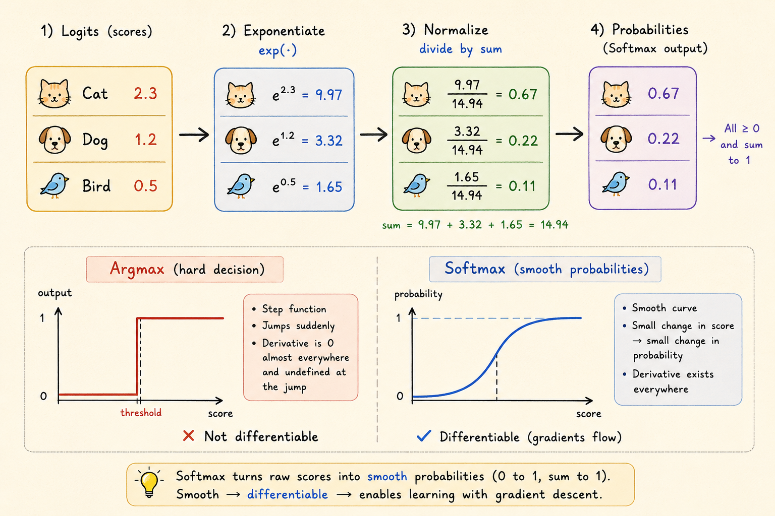
\[ \ell_{\mathrm{err}}(h(x), y) = \begin{cases} 0 & \text{if } \arg\max_i h_i(x) = y, \\ 1 & \text{otherwise}. \end{cases} \]
It is useful for evaluation, but it is a poor optimization objective because it is not differentiable.
Softmax / Cross-Entropy Loss
Softmax converts raw scores into a probability distribution:
\[ z_i = p(\text{label}=i) = \frac{\exp(h_i(x))} {\sum_{j=1}^{k}\exp(h_j(x))}. \]
The cross-entropy loss for the correct class \(y\) is
\[ \ell_{\mathrm{ce}}(h(x), y) = -\log p(\text{label}=y) = -h_y(x) + \log \sum_{j=1}^{k}\exp(h_j(x)). \]
Optimization
Softmax Regression Objective
The optimization goal is to minimize the average training loss:
\[ \min_\theta \frac{1}{m} \sum_{i=1}^{m} \ell(h_\theta(x^{(i)}), y^{(i)}). \]
For softmax regression:
\[ \min_\Theta \frac{1}{m} \sum_{i=1}^{m} \ell_{\mathrm{ce}}(\Theta^\top x^{(i)}, y^{(i)}). \]
Gradient Descent
The gradient \(\nabla_\theta f(\theta)\) has the same shape as the parameter matrix. It points in the direction of steepest local increase, so minimizing the loss means moving in the opposite direction:
\[ \theta := \theta - \alpha \nabla_\theta f(\theta). \]
Here \(\alpha\) is the learning rate.
Stochastic Gradient Descent
SGD estimates the full gradient with a minibatch of size \(B\):
\[ \theta := \theta - \frac{\alpha}{B} \sum_{i=1}^{B} \nabla_\theta \ell(h_\theta(x^{(i)}), y^{(i)}). \]
This gives more frequent parameter updates than waiting for a full pass over the training set.
Gradient of Softmax
For one example, the derivative of cross-entropy with respect to a score component \(h_i\) is
\[ \frac{\partial \ell_{\mathrm{ce}}(h,y)}{\partial h_i} = \frac{\partial}{\partial h_i} \left( -h_y + \log \sum_{j=1}^{k}\exp(h_j) \right). \]
The first term contributes \(-\mathbf{1}\{i=y\}\). The log-sum-exp term contributes the softmax probability:
\[ \frac{\partial}{\partial h_i} \log \sum_{j=1}^{k}\exp(h_j) = \frac{\exp(h_i)}{\sum_{j=1}^{k}\exp(h_j)} = z_i. \]
So the final component-wise gradient is
\[ \frac{\partial \ell_{\mathrm{ce}}(h,y)}{\partial h_i} = z_i - \mathbf{1}\{i=y\}. \]
In vector form:
\[ \nabla_h \ell_{\mathrm{ce}}(h,y) = z - e_y, \]
where \(z\) is the predicted probability vector and \(e_y\) is the one-hot vector for the true label.
Summary
For a minibatch \(X \in \mathbb{R}^{B \times n}\), softmax regression has a compact update:
\[ \Theta := \Theta - \frac{\alpha}{B} X^\top (Z - I_y). \]
Here \(Z\) is the minibatch matrix of predicted probabilities and \(I_y\) is the one-hot label matrix.
Key takeaways:
- The final algorithm is simple even though the derivation uses matrix calculus.
- Classification error is good for evaluation, while cross-entropy is better for gradient-based training.
- A basic linear softmax model can already reach less than 8% error on MNIST in a few seconds.
Source: CMU 10-414/714 Deep Learning Systems, Lecture 2: ML Refresher / Softmax Regression.