CMU Advanced NLP Lecture 21: Mixture of Experts
Mixture of Experts (MoE) replaces dense Transformer feed-forward layers with sparse expert layers. The model can have many parameters, but only a small subset is active for each token during training and inference.
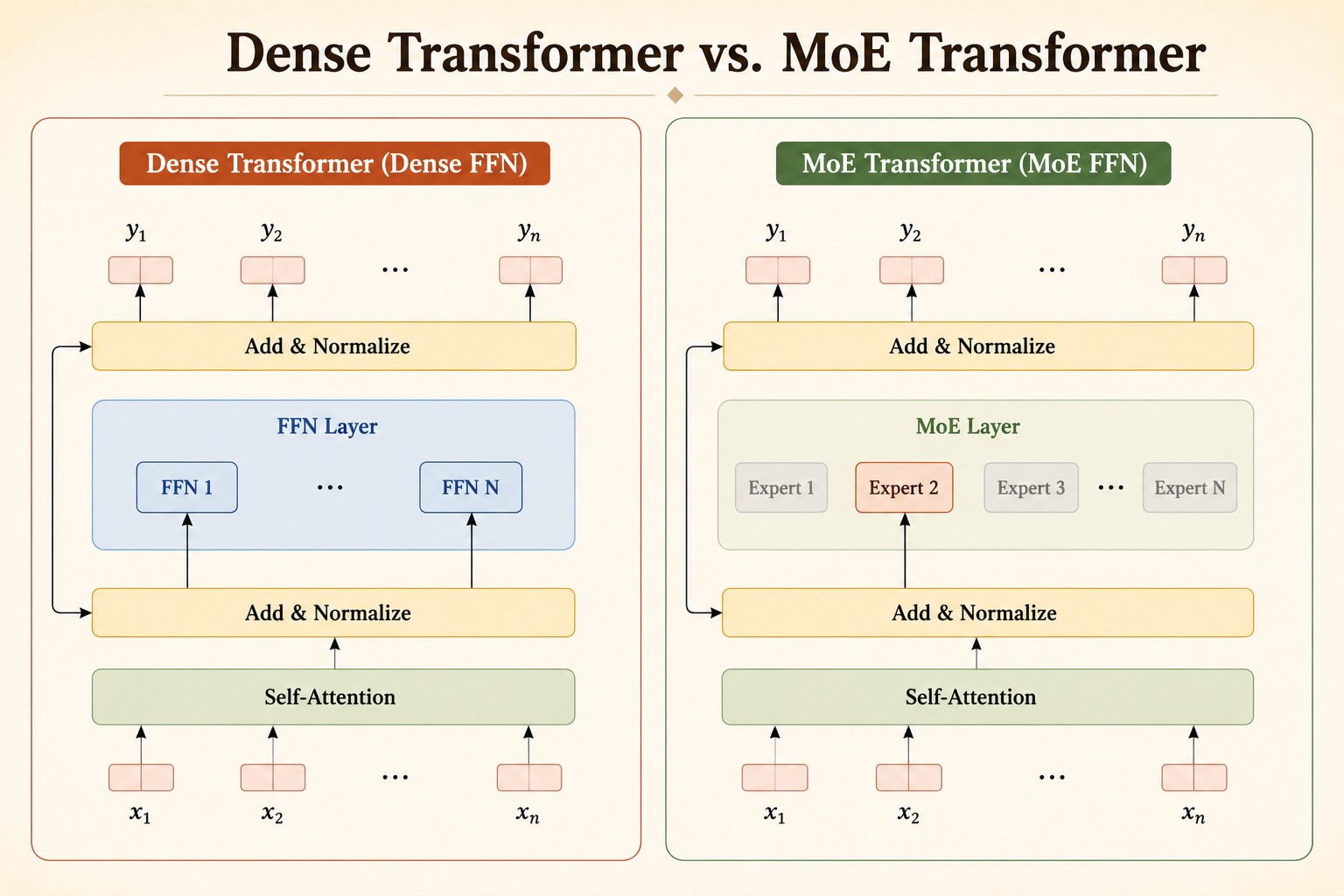
The core trade-off is:
- Scale parameter count while keeping active FLOPs roughly fixed.
- Reduce training compute compared with using an equally large dense FFN.
- Pay extra system complexity for routing, balancing, and communication.
Key Idea
An MoE layer is a neural network layer that activates only some of its parameters for each token. In modern LLMs, MoE is usually applied to the feed-forward layers inside Transformer blocks.
For a standard Transformer layer:
\[ \begin{aligned} \tilde{h}_{1:T} &= \operatorname{Attn}(h_{1:T}) + h_{1:T} \\ h'_{1:T} &= \operatorname{FFN}(\tilde{h}_{1:T}) + \tilde{h}_{1:T} \end{aligned} \]
For an MoE Transformer layer:
\[ \begin{aligned} \tilde{h}_{1:T} &= \operatorname{Attn}(h_{1:T}) + h_{1:T} \\ h'_{1:T} &= \operatorname{MoE}(\tilde{h}_{1:T}) + \tilde{h}_{1:T} \end{aligned} \]
The MoE module has two main pieces:
- Experts: \(N\) feed-forward networks, \(\operatorname{FFN}_1, \dots, \operatorname{FFN}_N\), each with its own parameters.
- Router: a learned function that selects one or more experts for each input token.
Expert Design
Where Experts Go
Most MoE language models place experts in the feed-forward layers.
- Typical: replace FFN layers with MoE layers.
- Less common: put experts in attention layers.
- Practical trend: use MoE in many or all FFN layers.
Attention experts can be unstable, while FFN experts are simpler and map naturally onto sparse computation.
Expert Count
Increasing the number of experts increases total parameters.
- More experts usually improve quality because the model has more specialized capacity.
- Gains eventually show diminishing returns.
- Active FLOPs can stay fixed, but total memory and parameter-management cost increase.
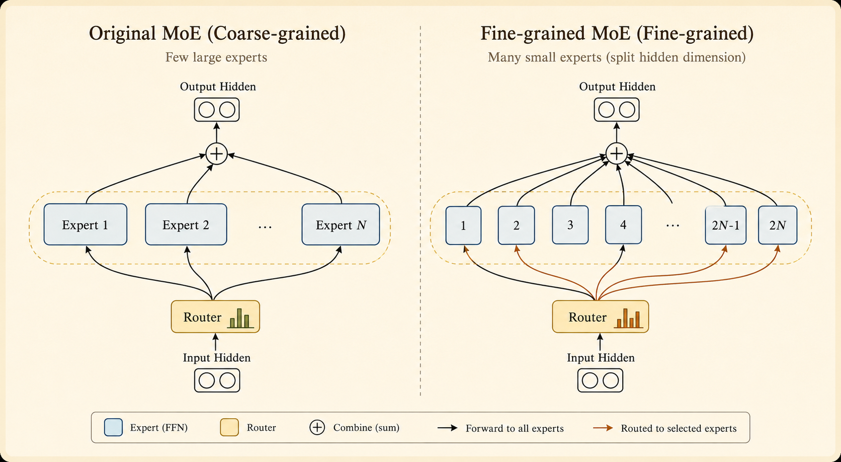
Fine-Grained Experts
Instead of using a few large experts, we can split the hidden dimension into smaller expert chunks.
- If each expert is smaller, the model can have more expert choices at similar total parameter count.
- More fine-grained experts give the router more possible expert combinations per token.
Routing Functions
Basic Idea
Routing computes a score for each token-expert pair.
- Token choice: each token selects its top-\(k\) experts. This is common in LLMs.
- Expert choice: each expert selects its top-\(k\) tokens. This guarantees more balanced expert load.
- Global choice: assignments are chosen by a batch-level optimization.
Computing Scores
Each expert has a learned weight vector \(e_i\). For token hidden state \(\tilde{h}_t\), the router computes:
\[ s_{t,i} = \operatorname{softmax}_i(\tilde{h}_t^T e_i) \]
Then the top-\(K\) experts are selected:
\[ g_{i,t} = \begin{cases} s_{t,i}, & i \in \operatorname{TopK}(\{s_{t,j} \mid 1 \le j \le N\}, K) \\ 0, & \text{otherwise} \end{cases} \]
The final output combines the selected experts with the residual connection:
\[ h'_t = \sum_{i=1}^{N} g_{i,t}\operatorname{FFN}_i(\tilde{h}_t) + \tilde{h}_t \]
Top-k Token Choice Routing
Top-k token choice is simple: each token chooses the experts with the highest routing scores.
Pros
- Every input token is assigned to at least one expert.
- The routing rule is simple to compute.
- It works well enough to be widely used.
Potential Issues
- Load imbalance: many tokens may choose the same expert.
- Token dropping: an overloaded expert may exceed capacity, forcing some tokens to skip that MoE layer.
- Non-differentiability: the top-k selection itself is discrete, which complicates training.
Alternative Routing Strategies
Expert Choice
Expert choice reverses the decision: each expert chooses a fixed number of tokens to process.
Benefits:
- It guarantees load balancing during training.
- It can allocate more computation to important or difficult tokens.
Costs:
- It does not naturally match autoregressive inference, where tokens arrive one at a time.
- A token may be ignored if no expert selects it.
Hash Routing
Hash routing removes the learned router. A deterministic hash function maps each token to an expert.
- Pros: no learned routing parameters and a surprisingly strong baseline.
- Cons: the router cannot adapt to data, so it is ultimately less flexible.
Reinforcement Learning Routing
Routing can also be framed as a decision problem: the router acts as a policy, expert selection is the action, and language-modeling quality provides the reward.
This is principled, but usually expensive and unstable:
- RL has high-variance gradients.
- It adds training overhead.
- At large scale, simpler top-k methods are often competitive enough to justify their use.
Auxiliary Losses
Balance Loss
Routers can collapse by sending too many tokens to the same expert. A balance loss penalizes this behavior:
\[ L = \alpha \sum_{i=1}^{N} f_i P_i \]
where:
- \(f_i\) is the fraction of tokens actually routed to expert \(i\).
- \(P_i\) is the average router probability assigned to expert \(i\).
- \(\alpha\) controls the strength of the balancing penalty.
The goal is to keep experts used more uniformly, which improves both model utilization and hardware utilization.
Z-Loss for Router Stability
Router logits can become numerically large, especially during large-scale training with lower precision formats such as BF16. The Z-loss penalizes large log-sum-exp values:
\[ L_Z(x) = \frac{1}{B} \sum_{i=1}^{B} \left( \log \sum_{j=1}^{N} e^{x_{i,j}} \right)^2 \]
Here \(x_{i,j}\) is the router logit for token \(i\) and expert \(j\). Penalizing the log partition term keeps router logits bounded and reduces numerical instability.
Expert Parallelism
Dense models usually use data parallelism or model parallelism. MoE adds another dimension: expert parallelism.
- Experts are placed on different devices.
- Tokens are dispatched to the devices that host their selected experts.
- Expert outputs are sent back and combined.
The benefit is memory scale: the model can contain many more parameters than a dense model with the same active FLOPs.
The cost is communication. Routing tokens to experts creates all-to-all traffic, so network bandwidth can become the bottleneck.
Takeaway
MoE is a way to scale model capacity without scaling active computation linearly. The hard part is not the basic idea; it is making sparse routing trainable, balanced, numerically stable, and efficient across devices.
Source: CMU Advanced NLP Fall 2025, Lecture 21: Mixture of Experts.