MIT 6.041 Probability: Iterated Expectations
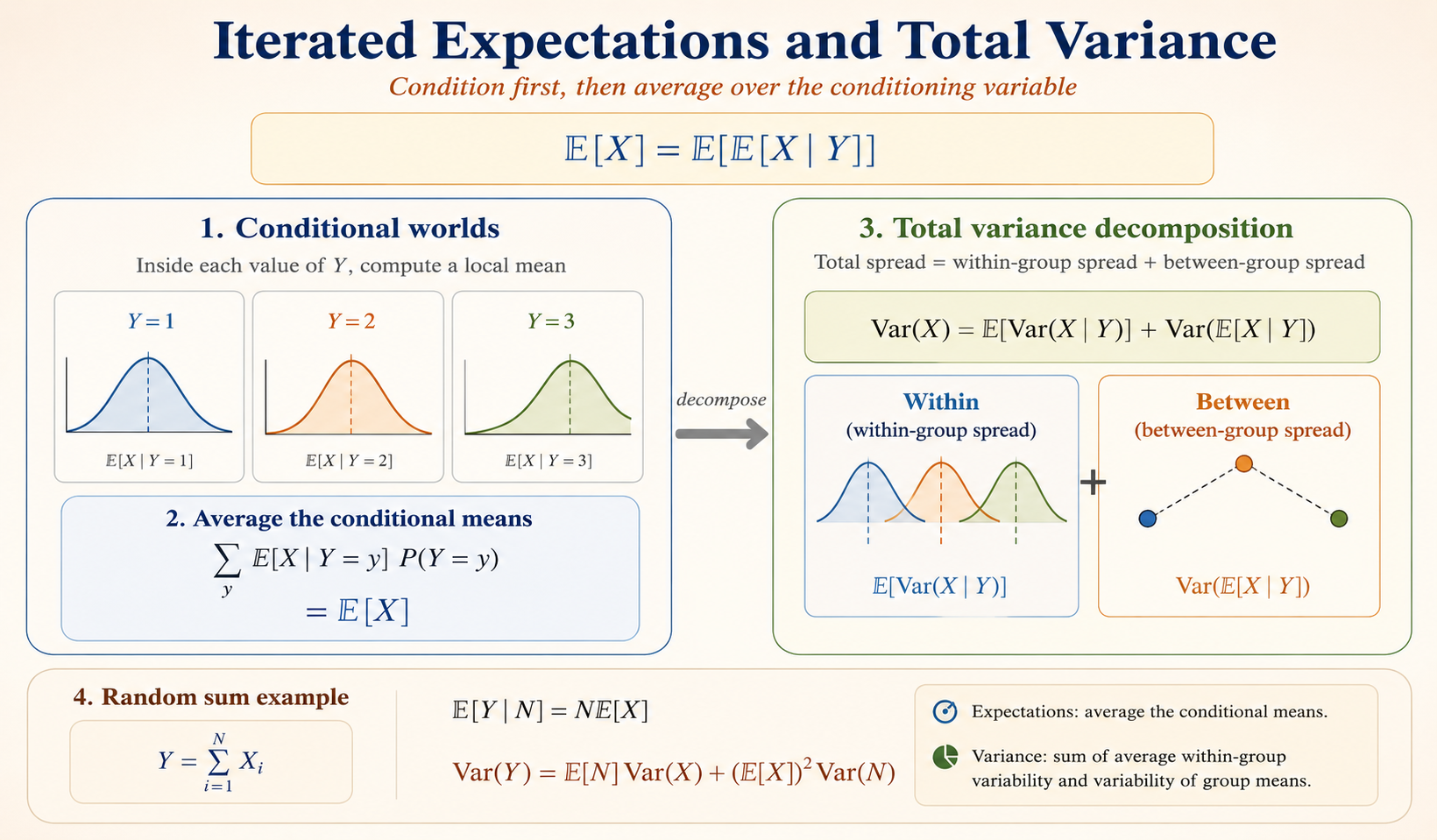
This lecture introduces one of the most useful habits in probability: condition first, solve the easier conditional problem, then average over the conditioning variable.
The same idea appears twice:
- for expectations, through the Law of Iterated Expectations
- for variances, through the Law of Total Variance
Law of Iterated Expectations
The Law of Iterated Expectations, also called the Law of Total Expectation, says that the unconditional expectation of \(X\) equals the expectation of the conditional expectation of \(X\) given \(Y\):
\[ \mathbb{E}[X] = \mathbb{E}\left[\mathbb{E}[X \mid Y]\right]. \]
The key idea is that we can first compute the average of \(X\) inside each conditional world \(Y=y\), then average those conditional means according to how likely each value of \(Y\) is.
Conditional Expectation as a Random Variable
The conditional expectation \(\mathbb{E}[X \mid Y]\) is itself a random variable because it is a function of \(Y\). We can write
\[ \mathbb{E}[X \mid Y] = g(Y). \]
If we are given a specific value \(Y=y\), the conditional expectation becomes a number:
\[ \mathbb{E}[X \mid Y=y] = g(y). \]
So \(\mathbb{E}[X \mid Y]\) changes with the random value of \(Y\), while \(\mathbb{E}[X \mid Y=y]\) is the fixed conditional mean for one group.
Summation Form
For a discrete random variable \(Y\),
\[ \mathbb{E}[g(Y)] = \sum_y g(y)P_Y(y). \]
Substituting \(g(y)=\mathbb{E}[X \mid Y=y]\) gives
\[ \mathbb{E}[X] = \sum_y \mathbb{E}[X \mid Y=y]P_Y(y). \]
This is often the easiest way to compute an expectation: split the sample space into cases, compute the conditional mean in each case, then weight by the probability of the case.
Law of Total Variance
The Law of Total Variance decomposes the total variance of \(X\) into two components:
\[ \operatorname{Var}(X) = \mathbb{E}\left[\operatorname{Var}(X \mid Y)\right] + \operatorname{Var}\left(\mathbb{E}[X \mid Y]\right). \]
The two terms have different meanings:
- \(\mathbb{E}[\operatorname{Var}(X \mid Y)]\) is the average variability within each conditional group.
- \(\operatorname{Var}(\mathbb{E}[X \mid Y])\) is the variability of the conditional means across groups.
So total variance is
\[ \text{total spread} = \text{average within-group spread} + \text{between-group spread}. \]
Proof
Start from the conditional variance identity:
\[ \operatorname{Var}(X \mid Y) = \mathbb{E}[X^2 \mid Y] - \left(\mathbb{E}[X \mid Y]\right)^2. \]
Taking expectation on both sides gives
\[ \mathbb{E}\left[\operatorname{Var}(X \mid Y)\right] = \mathbb{E}\left[\mathbb{E}[X^2 \mid Y]\right] - \mathbb{E}\left[\left(\mathbb{E}[X \mid Y]\right)^2\right]. \]
By iterated expectations,
\[ \mathbb{E}\left[\mathbb{E}[X^2 \mid Y]\right] = \mathbb{E}[X^2], \]
so
\[ \mathbb{E}\left[\operatorname{Var}(X \mid Y)\right] = \mathbb{E}[X^2] - \mathbb{E}\left[\left(\mathbb{E}[X \mid Y]\right)^2\right]. \tag{1} \]
Next, apply the variance identity to the random variable \(\mathbb{E}[X \mid Y]\):
\[ \operatorname{Var}\left(\mathbb{E}[X \mid Y]\right) = \mathbb{E}\left[\left(\mathbb{E}[X \mid Y]\right)^2\right] - \left(\mathbb{E}\left[\mathbb{E}[X \mid Y]\right]\right)^2. \]
Again by iterated expectations,
\[ \mathbb{E}\left[\mathbb{E}[X \mid Y]\right] = \mathbb{E}[X], \]
therefore
\[ \operatorname{Var}\left(\mathbb{E}[X \mid Y]\right) = \mathbb{E}\left[\left(\mathbb{E}[X \mid Y]\right)^2\right] - \left(\mathbb{E}[X]\right)^2. \tag{2} \]
Adding (1) and (2), the middle terms cancel:
\[ \mathbb{E}\left[\operatorname{Var}(X \mid Y)\right] + \operatorname{Var}\left(\mathbb{E}[X \mid Y]\right) = \mathbb{E}[X^2] - \left(\mathbb{E}[X]\right)^2. \]
The right-hand side is \(\operatorname{Var}(X)\), so
\[ \operatorname{Var}(X) = \mathbb{E}\left[\operatorname{Var}(X \mid Y)\right] + \operatorname{Var}\left(\mathbb{E}[X \mid Y]\right). \]
Example: Section Means and Variance
Suppose a class is divided into two sections. Pick a student at random.
- \(X\): the student’s quiz score.
- \(Y\): the section number.
Assume:
- Section 1 has 10 students, average score 90, and variance 10.
- Section 2 has 20 students, average score 60, and variance 20.
The global average score is
\[ \mathbb{E}[X] = \frac{90\cdot 10 + 60\cdot 20}{30} = 70. \]
The conditional means are
\[ \mathbb{E}[X \mid Y=1] = 90, \qquad \mathbb{E}[X \mid Y=2] = 60. \]
The between-group component is
\[ \operatorname{Var}\left(\mathbb{E}[X \mid Y]\right) = \frac{1}{3}(90-70)^2 + \frac{2}{3}(60-70)^2 = 200. \]
The within-group component is
\[ \mathbb{E}\left[\operatorname{Var}(X \mid Y)\right] = \frac{1}{3}\cdot 10 + \frac{2}{3}\cdot 20 = \frac{50}{3} \approx 16.67. \]
Therefore,
\[ \operatorname{Var}(X) = \frac{50}{3} + 200. \]
The total variance is large mainly because the two section averages are far apart.
Example: Sum of a Random Number of Variables
Let
\[ Y = \sum_{i=1}^{N} X_i, \]
where:
- \(N\) is a non-negative integer random variable.
- \(X_i\) is the amount spent in store \(i\).
- The \(X_i\) are i.i.d.
- The \(X_i\) are independent of \(N\).
Conditioning on \(N=n\) turns the random sum into a fixed-length sum:
\[ \mathbb{E}[Y \mid N=n] = \mathbb{E}\left[\sum_{i=1}^{n}X_i\right] = \sum_{i=1}^{n}\mathbb{E}[X_i] = n\mathbb{E}[X]. \]
Therefore,
\[ \mathbb{E}[Y \mid N] = N\mathbb{E}[X]. \]
Taking expectation again gives
\[ \mathbb{E}[Y] = \mathbb{E}[N]\mathbb{E}[X]. \]
For the variance, use total variance:
\[ \operatorname{Var}(Y) = \mathbb{E}\left[\operatorname{Var}(Y \mid N)\right] + \operatorname{Var}\left(\mathbb{E}[Y \mid N]\right). \]
If \(N=n\), then \(Y\) is the sum of \(n\) independent copies of \(X\), so
\[ \operatorname{Var}(Y \mid N=n) = n\operatorname{Var}(X). \]
Thus
\[ \mathbb{E}\left[\operatorname{Var}(Y \mid N)\right] = \mathbb{E}[N]\operatorname{Var}(X). \]
Also,
\[ \operatorname{Var}\left(\mathbb{E}[Y \mid N]\right) = \operatorname{Var}\left(N\mathbb{E}[X]\right) = \left(\mathbb{E}[X]\right)^2\operatorname{Var}(N). \]
Putting the two pieces together:
\[ \operatorname{Var}(Y) = \mathbb{E}[N]\operatorname{Var}(X) + \left(\mathbb{E}[X]\right)^2\operatorname{Var}(N). \]
The first term is the expected within-sum variability. The second term is the extra variability from not knowing how many terms will appear in the sum.