MIT 6.041 Probability: Derived Distributions and Covariance
This lecture continues derived distributions and then introduces covariance as a way to describe how two random variables move together.
Ratio of Two Uniform Random Variables
Let \(X\) and \(Y\) be independent uniform random variables on \([0,1]\):
\[ X, Y \sim \operatorname{Uniform}(0,1) \]
Define
\[ Z = \frac{Y}{X} \]
We want the PDF of \(Z\).
The CDF is
\[ F_Z(z) = P\left(\frac{Y}{X} \le z\right) = P(Y \le zX) \]
Since \((X,Y)\) is uniform on the unit square, this probability is the area of the region below the line \(Y=zX\) inside the square.
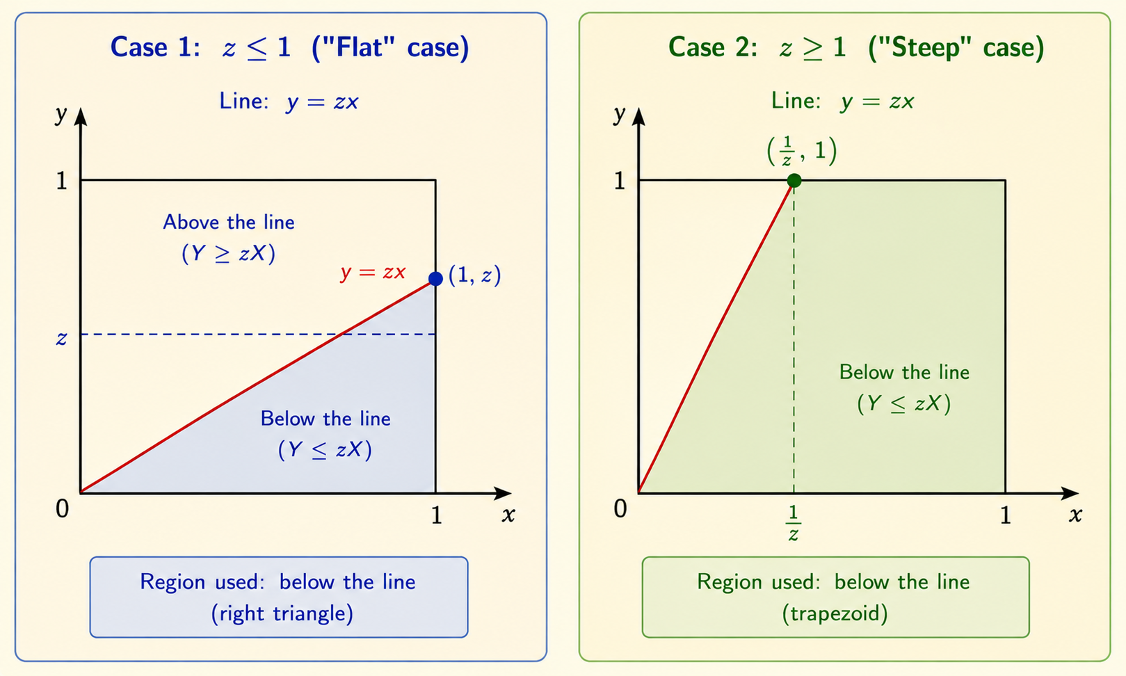
Case 1: \(0 \le z \le 1\)
The line \(Y=zX\) hits the right edge of the square at height \(z\). The region below the line is a triangle with base \(1\) and height \(z\):
\[ F_Z(z) = \frac{1}{2}\cdot 1 \cdot z = \frac{z}{2} \]
Differentiate:
\[ f_Z(z) = \frac{d}{dz}F_Z(z) = \frac{1}{2} \]
Case 2: \(z > 1\)
The line \(Y=zX\) is steep and hits the top edge of the square at
\[ X = \frac{1}{z} \]
It is easier to compute the complement. The small triangle above the line has base \(1/z\) and height \(1\):
\[ \text{Complement area} = \frac{1}{2}\cdot \frac{1}{z}\cdot 1 = \frac{1}{2z} \]
Therefore,
\[ F_Z(z) = 1 - \frac{1}{2z} \]
Differentiate:
\[ f_Z(z) = \frac{d}{dz}\left(1 - \frac{1}{2z}\right) = \frac{1}{2z^2} \]
So the PDF is
\[ f_Z(z) = \begin{cases} 0, & z < 0 \\ \frac{1}{2}, & 0 \le z \le 1 \\ \frac{1}{2z^2}, & z > 1 \end{cases} \]
Expectation of the Ratio
Using the PDF:
\[ E[Z] = \int_0^1 z\left(\frac{1}{2}\right)\,dz + \int_1^\infty z\left(\frac{1}{2z^2}\right)\,dz \]
The first part is finite:
\[ \int_0^1 \frac{z}{2}\,dz = \left[\frac{z^2}{4}\right]_0^1 = \frac{1}{4} \]
The second part diverges:
\[ \int_1^\infty \frac{1}{2z}\,dz = \frac{1}{2} \left[\ln z\right]_1^\infty = \infty \]
Therefore,
\[ E[Z] = \infty \]
The ratio has a heavy enough tail that its expectation does not exist as a finite number.
General Transformation Formula
Suppose
\[ Y = g(X) \]
where \(g\) is strictly monotonic. The key idea is conservation of probability: probability mass is preserved when we map a small interval of \(X\) into a small interval of \(Y\).
If \(y=g(x)\), then approximately:
\[ f_X(x)\,dx = f_Y(y)\,dy \]
Since
\[ dy = \left|g'(x)\right|dx \]
we get
\[ f_Y(y) = \frac{f_X(x)}{|g'(x)|} \]
where \(x = g^{-1}(y)\). Equivalently:
\[ f_Y(y) = f_X(g^{-1}(y)) \left| \frac{d}{dy}g^{-1}(y) \right| \]
This avoids recomputing the CDF when the transformation is one-to-one.
Convolution Formula
Let
\[ W = X + Y \]
Discrete Case
If \(X\) and \(Y\) are independent discrete random variables, then
\[ P(W=w) = \sum_x P(X=x)P(Y=w-x) \]
The sum runs over all values of \(x\) that make \(y=w-x\) possible.
Continuous Case
If \(X\) and \(Y\) are independent continuous random variables, then the PDF of their sum is the convolution:
\[ f_W(w) = \int_{-\infty}^{\infty} f_X(x)f_Y(w-x)\,dx \]
The convolution adds up all ways to split the total value \(w\) into one contribution from \(X\) and one from \(Y\).
Two Independent Normal Variables
If \(X\) and \(Y\) are independent, their joint PDF factors:
\[ f_{X,Y}(x,y) = f_X(x)f_Y(y) \]
For independent normal variables, the joint density has elliptical contours:
\[ \frac{(x-\mu_X)^2}{2\sigma_X^2} + \frac{(y-\mu_Y)^2}{2\sigma_Y^2} = \text{constant} \]
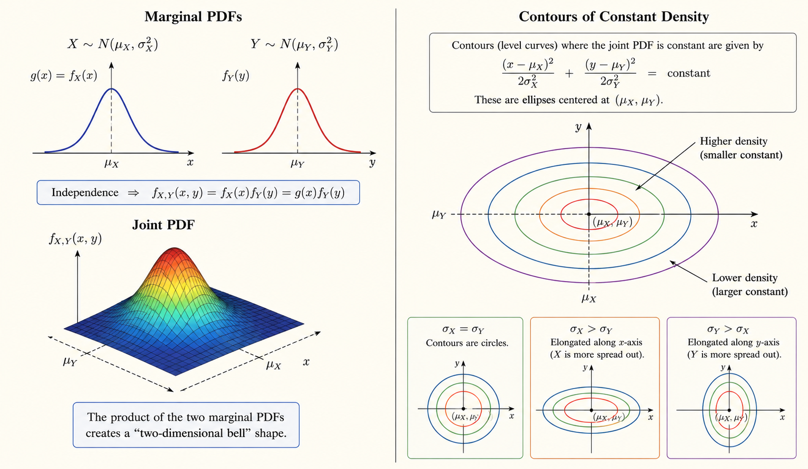
The ellipses are centered at \((\mu_X,\mu_Y)\). If \(\sigma_X=\sigma_Y\), the contours are circles. If one variance is larger, the contours stretch along that axis.
Sum of Independent Normals
If
\[ X \sim N(0,\sigma_X^2), \qquad Y \sim N(0,\sigma_Y^2) \]
and \(X\) and \(Y\) are independent, then
\[ W = X + Y \]
is also normal:
\[ W \sim N(0,\sigma_X^2+\sigma_Y^2) \]
More generally, means add and variances add for independent normal random variables.
Covariance
Covariance measures how two random variables vary together:
\[ \operatorname{cov}(X,Y) = E[(X-E[X])(Y-E[Y])] \]
The useful shortcut is
\[ \operatorname{cov}(X,Y) = E[XY] - E[X]E[Y] \]
If both variables have zero mean, then
\[ \operatorname{cov}(X,Y) = E[XY] \]
Interpretation:
- Positive covariance: large values of \(X\) tend to come with large values of \(Y\).
- Negative covariance: large values of \(X\) tend to come with small values of \(Y\).
- Zero covariance: no linear association, but not necessarily independence.
Variance of a Sum
For random variables \(X_1,\dots,X_n\):
\[ \operatorname{var}\left(\sum_{i=1}^n X_i\right) = \sum_{i=1}^n \operatorname{var}(X_i) + \sum_{(i,j):i\ne j} \operatorname{cov}(X_i,X_j) \]
If the variables are independent, all covariance terms are zero, so:
\[ \operatorname{var}\left(\sum_{i=1}^n X_i\right) = \sum_{i=1}^n \operatorname{var}(X_i) \]
Correlation Coefficient
The correlation coefficient standardizes covariance:
\[ \rho = \frac{\operatorname{cov}(X,Y)} {\sigma_X\sigma_Y} \]
Key properties:
- \(-1 \le \rho \le 1\).
- If \(|\rho|=1\), the variables have a perfect linear relationship.
- If \(X\) and \(Y\) are independent, then \(\rho=0\).
- But \(\rho=0\) does not imply independence; it only means there is no linear association.
Covariance gives the direction and scale of joint variation. Correlation gives a unitless measure of the strength of linear association.
Source: MIT 6.041 Probabilistic Systems Analysis and Applied Probability, Lecture 11: Derived Distributions (continued); Covariance.