CMU DLSys Lecture 3 Part II: Manual Neural Networks
Part I introduced neural networks as nonlinear hypothesis classes. Part II asks a systems-oriented question: if a network is just matrix operations and elementwise nonlinearities, how do we compute all gradients efficiently?
The answer is backpropagation: cache intermediate activations during the forward pass, then reuse local derivatives during a backward pass.
Gradients of a Two-Layer Network
Consider a simple two-layer network:
\[ Z = XW_1, \qquad H = \sigma(Z), \qquad U = HW_2, \qquad S = \operatorname{softmax}(U). \]
For cross-entropy loss with one-hot labels \(I_y\), the output-layer error is:
\[ G_U = \frac{\partial \ell_{\text{ce}}}{\partial U} = S - I_y. \]
Here:
- \(S\) is the predicted probability distribution.
- \(I_y\) is the one-hot ground-truth label.
- \(S - I_y\) is the error signal at the logits.
For example:
\[ S = \begin{bmatrix} 0.2 \\ 0.6 \\ 0.2 \end{bmatrix}, \qquad I_y = \begin{bmatrix} 0 \\ 1 \\ 0 \end{bmatrix}, \qquad S - I_y = \begin{bmatrix} 0.2 \\ -0.4 \\ 0.2 \end{bmatrix}. \]
Gradient With Respect to \(W_2\)
The second layer is:
\[ U = HW_2. \]
Because \(H\) is the input to this linear layer, the weight gradient is:
\[ \nabla_{W_2}\ell_{\text{ce}} = H^T G_U = H^T(S - I_y). \]
This is the same pattern as linear classification: input activations transposed times output error.
Gradient With Respect to \(W_1\)
For the first layer, the gradient must pass through:
\[ W_2, \qquad \sigma, \qquad XW_1. \]
By the chain rule:
\[ \frac{\partial \ell_{\text{ce}}}{\partial W_1} = \frac{\partial \ell_{\text{ce}}}{\partial U} \frac{\partial U}{\partial H} \frac{\partial H}{\partial Z} \frac{\partial Z}{\partial W_1}. \]
In matrix form:
\[ \nabla_{W_1}\ell_{\text{ce}} = X^T \left( \left((S - I_y)W_2^T\right) \circ \sigma'(XW_1) \right). \]
The components are:
- \(X^T\): input activations transposed.
- \((S - I_y)W_2^T\): output error propagated backward through \(W_2\).
- \(\circ \sigma'(XW_1)\): elementwise multiplication by the activation derivative.
Backpropagation in General
For a fully connected network, write each layer as:
\[ Z_{i+1} = \sigma_i(Z_i W_i), \qquad i = 1, \dots, L. \]
The gradient of the loss with respect to one weight matrix \(W_i\) can be written as a long chain:
\[ \frac{\partial \ell(Z_{L+1}, y)}{\partial W_i} = \frac{\partial \ell}{\partial Z_{L+1}} \frac{\partial Z_{L+1}}{\partial Z_L} \cdots \frac{\partial Z_{i+2}}{\partial Z_{i+1}} \frac{\partial Z_{i+1}}{\partial W_i}. \]
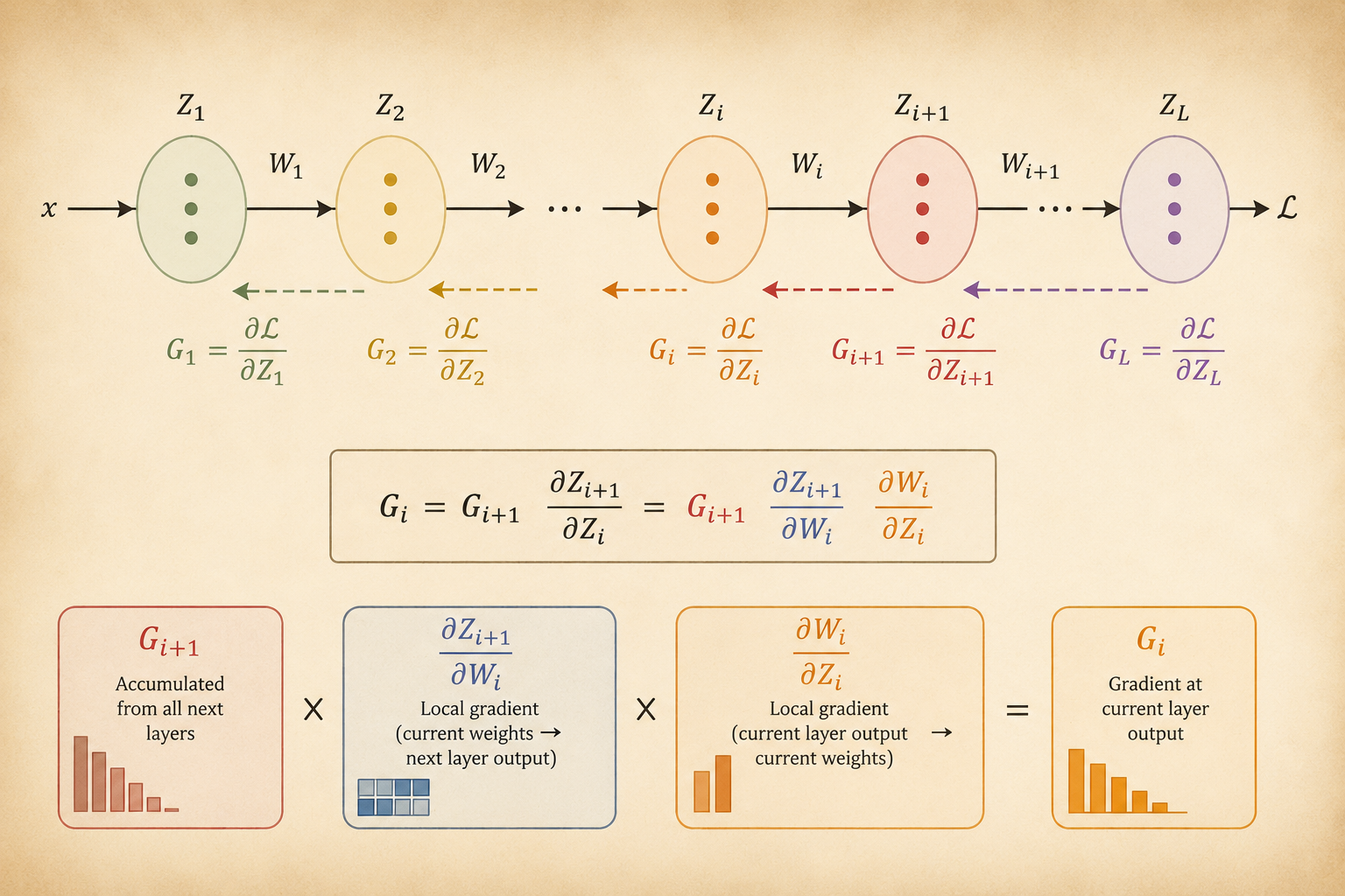
Naively computing this full product separately for every layer would be wasteful. Backpropagation reuses the accumulated gradient from later layers.
Define the upstream gradient:
\[ G_{i+1} = \frac{\partial \ell(Z_{L+1}, y)}{\partial Z_{i+1}}. \]
Then the backward recursion is:
\[ G_i = G_{i+1} \frac{\partial Z_{i+1}}{\partial Z_i}. \]
In practice, we do not explicitly materialize huge Jacobian matrices. Each layer implements the corresponding vector-Jacobian product.
Matrix Backpropagation
For the layer:
\[ Z_{i+1} = \sigma_i(Z_i W_i), \]
define:
\[ A_i = Z_i W_i. \]
The gradient with respect to the layer input is:
\[ G_i = \left( G_{i+1} \circ \sigma_i'(A_i) \right) W_i^T. \]
The gradient with respect to the weight matrix is:
\[ \nabla_{W_i}\ell = Z_i^T \left( G_{i+1} \circ \sigma_i'(A_i) \right). \]
The same local error term appears in both equations:
\[ G_{i+1} \circ \sigma_i'(A_i). \]
This term combines the incoming gradient from later layers with the derivative of the current activation.
Forward and Backward Passes
Forward Pass
The forward pass computes and caches activations.
- Set \(Z_1 = X\).
- For each layer, compute:
\[ Z_{i+1} = \sigma_i(Z_i W_i), \qquad i = 1, \dots, L. \]
The cache stores values such as \(Z_i\) and \(A_i = Z_iW_i\), which are needed during the backward pass.
Backward Pass
The backward pass propagates the loss gradient from output to input.
- Initialize the final gradient. For softmax cross-entropy:
\[ G_{L+1} = \nabla_{Z_{L+1}}\ell(Z_{L+1}, y) = S - I_y. \]
- Iterate backward for \(i = L, \dots, 1\):
\[ G_i = \left( G_{i+1} \circ \sigma_i'(Z_iW_i) \right) W_i^T. \]
- Compute each weight gradient:
\[ \nabla_{W_i}\ell = Z_i^T \left( G_{i+1} \circ \sigma_i'(Z_iW_i) \right). \]
Takeaways
- Backpropagation is the chain rule organized for reuse.
- \(G_{i+1}\) is the accumulated upstream gradient from later layers.
- Each layer only needs its local derivative and cached forward values.
- The key systems primitive is the vector-Jacobian product, not explicit Jacobian construction.
- This modular view is what makes automatic differentiation possible for larger computation graphs.
Source: CMU 10-414/714 Deep Learning Systems, Lecture 3 Part II: Manual Neural Networks.