MIT 6.041 Probability: Bernoulli Process
A Bernoulli process is the simplest discrete-time arrival model: at every time slot, the same independent experiment is repeated.
Each trial has
\[ P(X_i = 1) = p, \qquad P(X_i = 0) = 1-p. \]
Here \(X_i=1\) means success or arrival in slot \(i\), while \(X_i=0\) means failure or no arrival.
Definition
A Bernoulli process is a sequence
\[ X_1, X_2, X_3, \ldots \]
where the random variables are independent and identically distributed Bernoulli random variables with parameter \(p\).
Examples:
- lottery win/loss outcomes across repeated plays
- daily up/down movements of a stock index
- arrivals in discrete time slots, where \(1\) means someone arrives and \(0\) means no one arrives
Basic Properties
For a Bernoulli random variable \(X\) with parameter \(p\),
\[ \mathbb{E}[X] = 1\cdot p + 0\cdot(1-p) = p. \]
Because \(X^2=X\) for \(X\in\{0,1\}\),
\[ \mathbb{E}[X^2] = p. \]
Therefore,
\[ \operatorname{Var}(X) = \mathbb{E}[X^2] - \left(\mathbb{E}[X]\right)^2 = p-p^2 = p(1-p). \]
The Bernoulli process is memoryless in discrete time: knowing previous outcomes does not change the distribution of future outcomes. Even after a long streak of failures, the next trial still has success probability \(p\).
This is the discrete-time analogue of the Poisson process, which is memoryless in continuous time.
Number of Successes in Fixed Time
Let
\[ S_n = X_1 + X_2 + \cdots + X_n \]
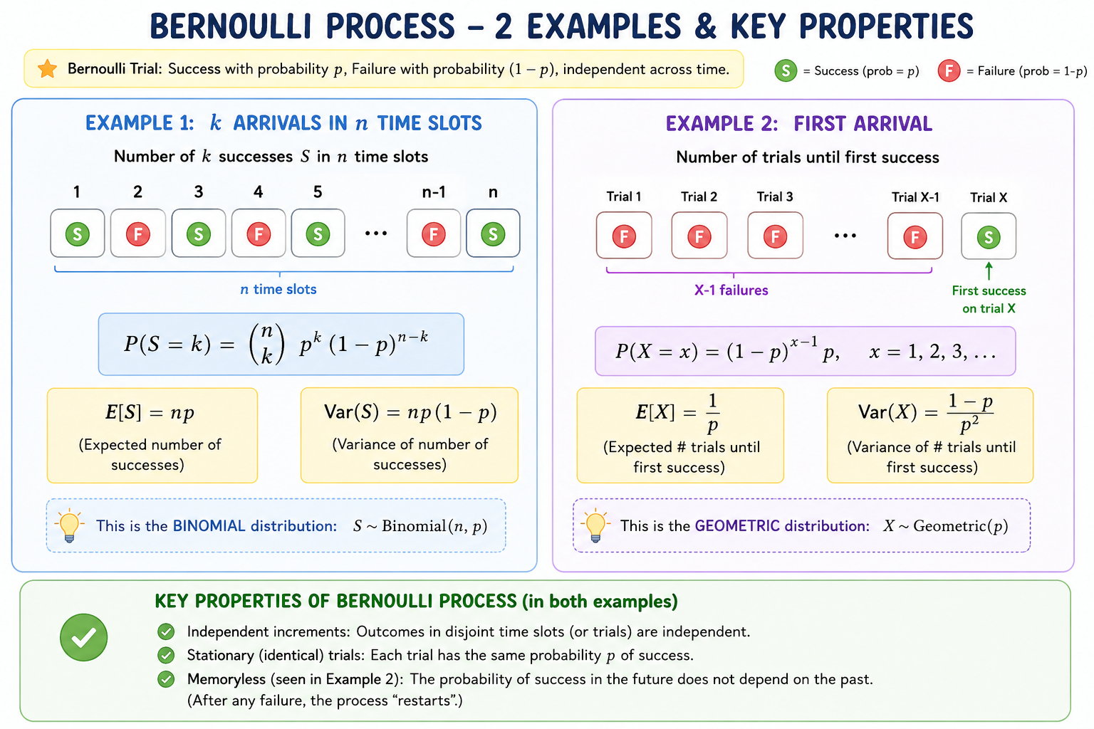
be the number of successes in the first \(n\) slots. Then \(S_n\) follows a binomial distribution:
\[ P(S_n=k) = \binom{n}{k}p^k(1-p)^{n-k}. \]
Its expectation and variance are
\[ \mathbb{E}[S_n] = np, \qquad \operatorname{Var}(S_n) = np(1-p). \]
The intuition is direct: \(S_n\) adds \(n\) independent Bernoulli indicators.
First Arrival Time
Let \(T_1\) be the number of trials until the first success. To have the first success at time \(t\), the first \(t-1\) trials must fail and trial \(t\) must succeed:
\[ P(T_1=t) = (1-p)^{t-1}p, \qquad t=1,2,\ldots \]
So \(T_1\) follows a geometric distribution with
\[ \mathbb{E}[T_1] = \frac{1}{p}, \qquad \operatorname{Var}(T_1) = \frac{1-p}{p^2}. \]
Time of the \(k^{\text{th}}\) Success
Let \(Y_k\) be the time of the \(k^{\text{th}}\) success. For the \(k^{\text{th}}\) success to happen exactly at time \(t\):
- there must be exactly \(k-1\) successes in the first \(t-1\) trials
- trial \(t\) must be a success
Thus,
\[ P(Y_k=t) = \binom{t-1}{k-1}p^k(1-p)^{t-k}, \qquad t\ge k. \]
This is the negative binomial waiting-time distribution.
We can also view \(Y_k\) as the sum of \(k\) independent geometric waiting times:
\[ Y_k = T_1 + T_2 + \cdots + T_k. \]
Therefore,
\[ \mathbb{E}[Y_k] = \frac{k}{p}, \qquad \operatorname{Var}(Y_k) = \frac{k(1-p)}{p^2}. \]
For example, if one arrival takes \(10\) minutes on average, then three arrivals take \(30\) minutes on average.
Splitting
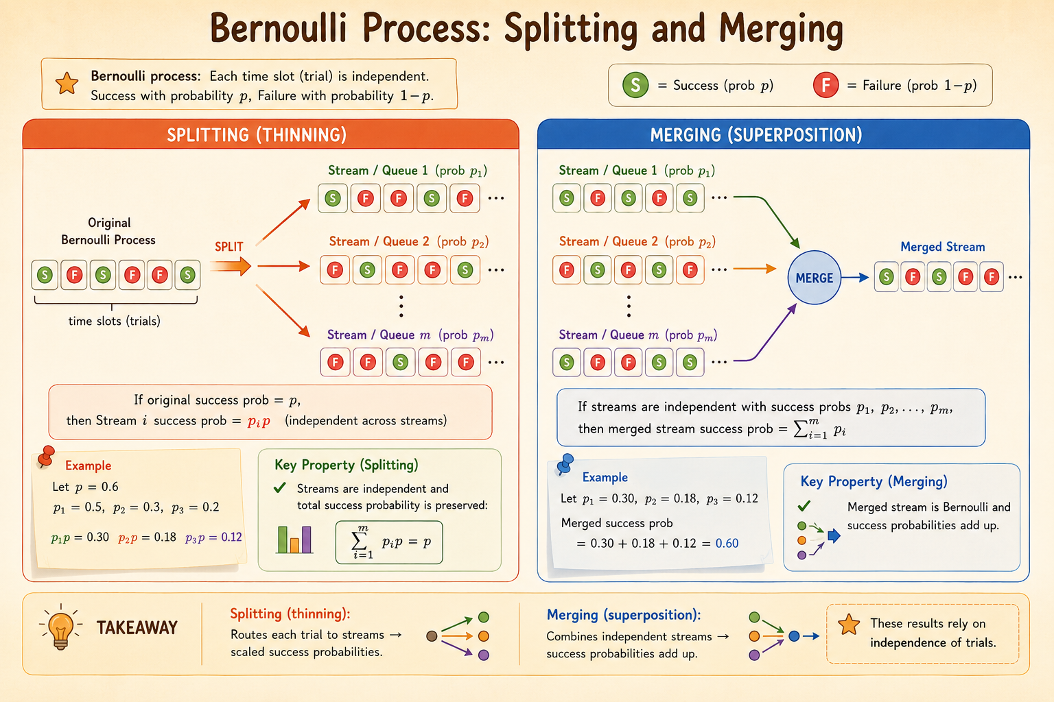
Suppose arrivals follow a Bernoulli process with arrival probability \(p\) in each time slot. Each arrival is then independently routed to Server 1 with probability \(q\) and to Server 2 with probability \(1-q\).
For Server 1 to see an arrival in a slot:
- an arrival must occur in the original process, probability \(p\)
- the arrival must be routed to Server 1, probability \(q\)
So Server 1 sees a Bernoulli process with probability
\[ pq. \]
Similarly, Server 2 sees a Bernoulli process with probability
\[ p(1-q). \]
Each split stream is Bernoulli across time, because the original arrivals and routing decisions are independent across slots.
Merging
Now suppose there are two independent Bernoulli arrival streams:
- Stream 1 has arrival probability \(p\)
- Stream 2 has arrival probability \(q\)
The merged process records \(1\) if at least one stream has an arrival in the slot, and \(0\) otherwise.
It is easier to compute the probability of no arrival:
\[ P(\text{no arrival}) = (1-p)(1-q). \]
Therefore, the merged arrival probability is
\[ 1-(1-p)(1-q) = p+q-pq. \]
So the merged stream is also a Bernoulli process, with parameter \(p+q-pq\).
Takeaways
- A Bernoulli process is an independent sequence of success/failure trials.
- Counts in a fixed number of slots follow a binomial distribution.
- Waiting time until the first success follows a geometric distribution.
- Waiting time until the \(k^{\text{th}}\) success follows a negative binomial distribution.
- Splitting and merging preserve the Bernoulli-process structure, but change the success probability.
Source: MIT 6.041 Probabilistic Systems Analysis and Applied Probability, Bernoulli Process.