The Math Behind Quantum Entanglement
Main Idea
Entanglement is often described in physical language, but this note focuses on the mathematical meaning.
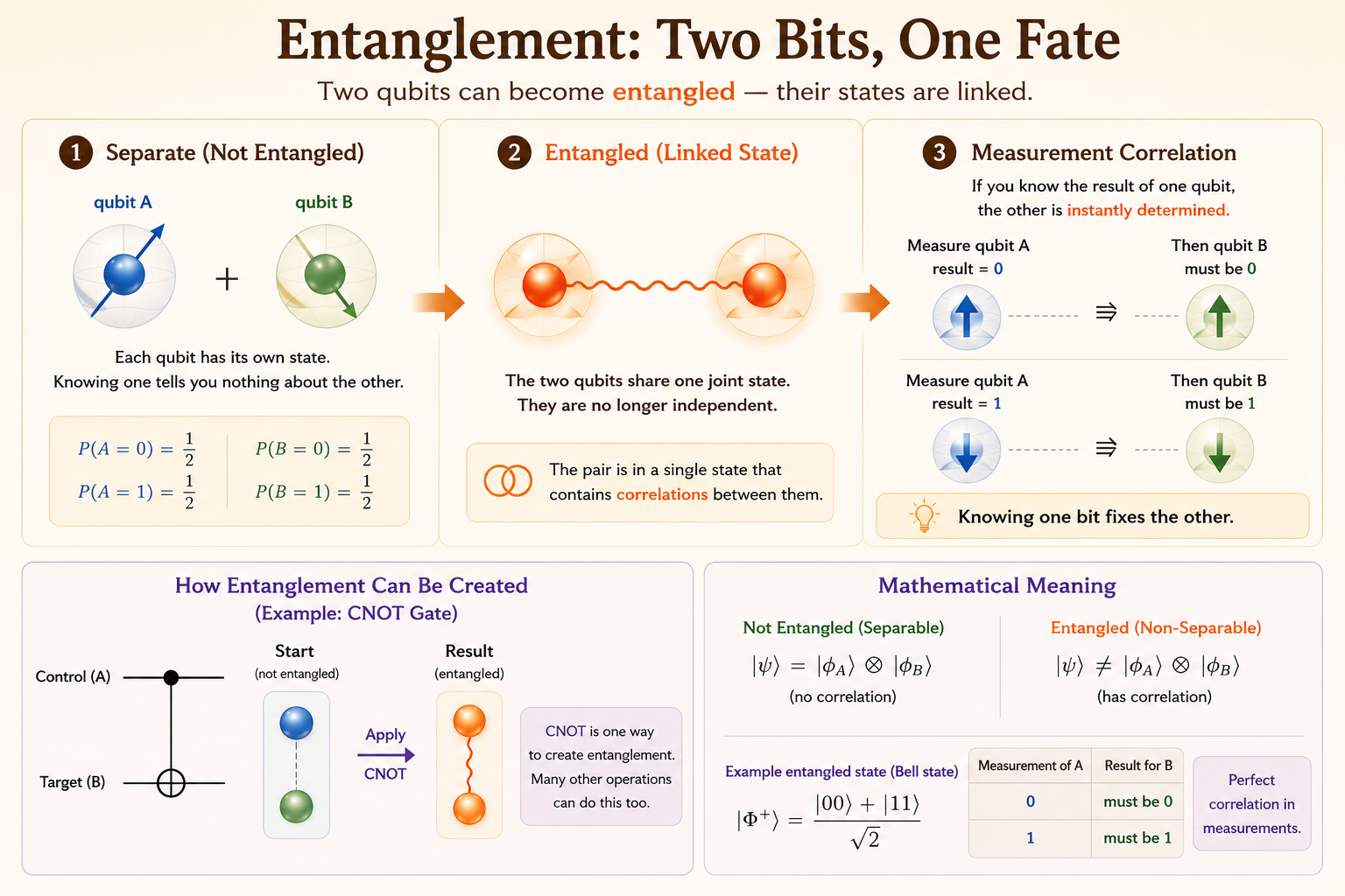
Mathematically, entanglement means the joint state of multiple qubits cannot be written as a simple product of independent single-qubit states. The two qubits must be described together as one shared state vector.
Qubit Collapse and Measurement
- The phrase “a qubit can exist in two positions at the same time” is misleading.
- In physics, there is no way to deterministically predict the measured position of a qubit.
- We can calculate the probability of a qubit being measured in each position.
- We can measure the qubit and get one position: the random position observed at measurement time.
Mathematically, a qubit state assigns amplitudes to possible measurement outcomes. Before measurement, we use the amplitudes to calculate probabilities. After measurement, we observe one outcome.
For a one-qubit state
\[ \lvert \psi \rangle = \alpha \lvert 0 \rangle + \beta \lvert 1 \rangle, \]
the probabilities are
\[ P(0) = |\alpha|^2, \qquad P(1) = |\beta|^2, \qquad |\alpha|^2 + |\beta|^2 = 1. \]
So quantum mechanics predicts the probability distribution of measurement results, not a deterministic outcome before measurement.
Bell State
A Bell state is a maximally entangled two-qubit state. The standard example is
\[ \lvert \Phi^+ \rangle = \frac{1}{\sqrt{2}}(\lvert 00 \rangle + \lvert 11 \rangle). \]
This state says there are only two possible outcomes:
- \(\lvert 00 \rangle\) with probability \(\frac{1}{2}\)
- \(\lvert 11 \rangle\) with probability \(\frac{1}{2}\)
The outcomes \(\lvert 01 \rangle\) and \(\lvert 10 \rangle\) have probability zero.
In vector form, using the basis order
\[ \lvert 00 \rangle,\ \lvert 01 \rangle,\ \lvert 10 \rangle,\ \lvert 11 \rangle, \]
the Bell state is
\[ \lvert \Phi^+ \rangle = \frac{1}{\sqrt{2}} \begin{bmatrix} 1 \\ 0 \\ 0 \\ 1 \end{bmatrix}. \]
What Entanglement Means Mathematically
The key question is whether the two-qubit Bell state can be separated into two one-qubit states.
Assume it could be written as
\[ (\alpha \lvert 0 \rangle + \beta \lvert 1 \rangle) \otimes (\gamma \lvert 0 \rangle + \delta \lvert 1 \rangle). \]
Expanding the tensor product gives
\[ \alpha\gamma \lvert 00 \rangle + \alpha\delta \lvert 01 \rangle + \beta\gamma \lvert 10 \rangle + \beta\delta \lvert 11 \rangle. \]
To match the Bell state, the coefficients would need to satisfy
\[ \alpha\gamma = \frac{1}{\sqrt{2}}, \qquad \alpha\delta = 0, \qquad \beta\gamma = 0, \qquad \beta\delta = \frac{1}{\sqrt{2}}. \]
This is impossible. The first equation requires both \(\alpha\) and \(\gamma\) to be nonzero. The last equation requires both \(\beta\) and \(\delta\) to be nonzero. But then \(\alpha\delta\) and \(\beta\gamma\) cannot both be zero.
That is the mathematical meaning of entanglement: the combined state cannot be factored into independent local states.
Gates
A quantum gate is a matrix that transforms one state vector into another state vector.
This section explains entanglement from the mathematical side: how gate operations change quantum state vectors and create correlated measurement outcomes. It is not a physics explanation of what physically causes entanglement.
Single-Qubit Gate: Hadamard
The Hadamard gate is
\[ H = \frac{1}{\sqrt{2}} \begin{bmatrix} 1 & 1 \\ 1 & -1 \end{bmatrix}. \]
Applied to \(\lvert 0 \rangle\), it creates an equal superposition:
\[ H \lvert 0 \rangle = \frac{1}{\sqrt{2}} \begin{bmatrix} 1 & 1 \\ 1 & -1 \end{bmatrix} \begin{bmatrix} 1 \\ 0 \end{bmatrix} = \frac{1}{\sqrt{2}} \begin{bmatrix} 1 \\ 1 \end{bmatrix} = \frac{1}{\sqrt{2}}(\lvert 0 \rangle + \lvert 1 \rangle). \]
Applied to \(\lvert 1 \rangle\), it creates
\[ H \lvert 1 \rangle = \frac{1}{\sqrt{2}} \begin{bmatrix} 1 & 1 \\ 1 & -1 \end{bmatrix} \begin{bmatrix} 0 \\ 1 \end{bmatrix} = \frac{1}{\sqrt{2}} \begin{bmatrix} 1 \\ -1 \end{bmatrix} = \frac{1}{\sqrt{2}}(\lvert 0 \rangle - \lvert 1 \rangle). \]
Two-Qubit Gate: CNOT
The CNOT gate flips the target qubit if the control qubit is 1.
Using the basis order
\[ \lvert 00 \rangle,\ \lvert 01 \rangle,\ \lvert 10 \rangle,\ \lvert 11 \rangle, \]
its matrix is
\[ \operatorname{CNOT} = \begin{bmatrix} 1 & 0 & 0 & 0 \\ 0 & 1 & 0 & 0 \\ 0 & 0 & 0 & 1 \\ 0 & 0 & 1 & 0 \end{bmatrix}. \]
The action on basis states is:
| Input | Output | Meaning |
|---|---|---|
| \(\lvert 00 \rangle\) | \(\lvert 00 \rangle\) | Control is 0, target unchanged |
| \(\lvert 01 \rangle\) | \(\lvert 01 \rangle\) | Control is 0, target unchanged |
| \(\lvert 10 \rangle\) | \(\lvert 11 \rangle\) | Control is 1, target flips from 0 to 1 |
| \(\lvert 11 \rangle\) | \(\lvert 10 \rangle\) | Control is 1, target flips from 1 to 0 |
Basis-State Calculations
For \(\lvert 00 \rangle\):
\[ \operatorname{CNOT}\lvert 00 \rangle = \begin{bmatrix} 1 & 0 & 0 & 0 \\ 0 & 1 & 0 & 0 \\ 0 & 0 & 0 & 1 \\ 0 & 0 & 1 & 0 \end{bmatrix} \begin{bmatrix} 1 \\ 0 \\ 0 \\ 0 \end{bmatrix} = \begin{bmatrix} 1 \\ 0 \\ 0 \\ 0 \end{bmatrix} = \lvert 00 \rangle. \]
For \(\lvert 01 \rangle\):
\[ \operatorname{CNOT}\lvert 01 \rangle = \begin{bmatrix} 1 & 0 & 0 & 0 \\ 0 & 1 & 0 & 0 \\ 0 & 0 & 0 & 1 \\ 0 & 0 & 1 & 0 \end{bmatrix} \begin{bmatrix} 0 \\ 1 \\ 0 \\ 0 \end{bmatrix} = \begin{bmatrix} 0 \\ 1 \\ 0 \\ 0 \end{bmatrix} = \lvert 01 \rangle. \]
For \(\lvert 10 \rangle\):
\[ \operatorname{CNOT}\lvert 10 \rangle = \begin{bmatrix} 1 & 0 & 0 & 0 \\ 0 & 1 & 0 & 0 \\ 0 & 0 & 0 & 1 \\ 0 & 0 & 1 & 0 \end{bmatrix} \begin{bmatrix} 0 \\ 0 \\ 1 \\ 0 \end{bmatrix} = \begin{bmatrix} 0 \\ 0 \\ 0 \\ 1 \end{bmatrix} = \lvert 11 \rangle. \]
For \(\lvert 11 \rangle\):
\[ \operatorname{CNOT}\lvert 11 \rangle = \begin{bmatrix} 1 & 0 & 0 & 0 \\ 0 & 1 & 0 & 0 \\ 0 & 0 & 0 & 1 \\ 0 & 0 & 1 & 0 \end{bmatrix} \begin{bmatrix} 0 \\ 0 \\ 0 \\ 1 \end{bmatrix} = \begin{bmatrix} 0 \\ 0 \\ 1 \\ 0 \end{bmatrix} = \lvert 10 \rangle. \]
Creating a Bell State
Start with two qubits in \(\lvert 00 \rangle\).
Apply a Hadamard gate to the first qubit:
\[ \lvert 00 \rangle \xrightarrow{H \otimes I} \frac{1}{\sqrt{2}}(\lvert 00 \rangle + \lvert 10 \rangle). \]
Then apply CNOT with the first qubit as control:
\[ \frac{1}{\sqrt{2}}(\lvert 00 \rangle + \lvert 10 \rangle) \xrightarrow{\operatorname{CNOT}} \frac{1}{\sqrt{2}}(\lvert 00 \rangle + \lvert 11 \rangle). \]
The Hadamard gate creates superposition. The CNOT gate spreads that superposition across two qubits, producing a joint state where the two measurement outcomes are perfectly correlated.
Takeaways
- A qubit state stores amplitudes; squared amplitudes give measurement probabilities.
- A Bell state is a joint two-qubit state with perfectly correlated outcomes.
- The mathematical signature of entanglement is non-separability: the joint state cannot be factored into independent single-qubit states.
- Gates are matrices, and entanglement can be studied by tracking how those matrices transform state vectors.