MIT 6.041 Probability: Poisson Process I
A Poisson process is a continuous-time model for random arrivals.
It is the continuous analogue of a Bernoulli process: instead of checking whether an arrival happens in each discrete slot, we count arrivals over continuous time intervals.
Definition
Let \(N(t)\) be the number of arrivals by time \(t\). For an interval of length \(\tau\),
\[ P(k,\tau) = \Pr(N(t+\tau)-N(t)=k). \]
The process is characterized by three ideas:
- Homogeneity: the distribution depends only on the interval length \(\tau\), not on where the interval starts.
- Independent increments: numbers of arrivals in disjoint intervals are independent.
- Small-interval behavior: in a tiny interval, either no arrival happens or one arrival happens; two or more arrivals are negligible.
For a fixed interval length \(\tau\),
\[ \sum_{k=0}^{\infty} P(k,\tau)=1. \]
Small Interval Probabilities
For a very small interval of length \(\delta\),
\[ P(k,\delta) \approx \begin{cases} 1-\lambda\delta, & k=0,\\ \lambda\delta, & k=1,\\ 0, & k>1. \end{cases} \]
Here \(\lambda\) is the arrival rate per unit time.
Intuition:
- \(\lambda\delta\) is the approximate probability of one arrival in a tiny interval.
- \(1-\lambda\delta\) is the approximate probability of no arrival.
- The probability of more than one arrival in a tiny interval is approximately zero.
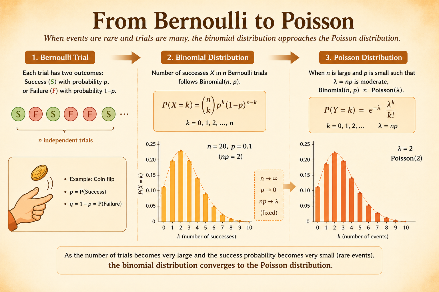
From Bernoulli to Poisson
The Poisson PMF can be derived as a limit of binomial probabilities.
Step 1: Discretize Time
Take an interval of length \(\tau\) and divide it into \(n\) small slots:
\[ \delta = \frac{\tau}{n}. \]
As \(n\to\infty\), the slot length \(\delta\to 0\).
Step 2: Match the Arrival Rate
Approximate each small slot as a Bernoulli trial with success probability
\[ p = \lambda\delta = \lambda\left(\frac{\tau}{n}\right) = \frac{\lambda\tau}{n}. \]
Then the expected number of arrivals in the whole interval is
\[ np = n\left(\frac{\lambda\tau}{n}\right) = \lambda\tau. \]
Step 3: Start from the Binomial PMF
If the \(n\) tiny slots are independent Bernoulli trials, then
\[ P(K_n=k) = \binom{n}{k}p^k(1-p)^{n-k}. \]
Substitute \(p=\lambda\tau/n\):
\[ P(K_n=k) = \binom{n}{k} \left(\frac{\lambda\tau}{n}\right)^k \left(1-\frac{\lambda\tau}{n}\right)^{n-k}. \]
Step 4: Take the Limit
For fixed \(k\),
\[ \binom{n}{k} = \frac{n(n-1)\cdots(n-k+1)}{k!}. \]
So
\[ P(K_n=k) = \frac{n(n-1)\cdots(n-k+1)}{k!} \left(\frac{\lambda\tau}{n}\right)^k \left(1-\frac{\lambda\tau}{n}\right)^n \left(1-\frac{\lambda\tau}{n}\right)^{-k}. \]
As \(n\to\infty\):
\[ \frac{n(n-1)\cdots(n-k+1)}{n^k}\to 1, \]
\[ \left(1-\frac{\lambda\tau}{n}\right)^n \to e^{-\lambda\tau}, \]
and
\[ \left(1-\frac{\lambda\tau}{n}\right)^{-k}\to 1. \]
Therefore,
\[ P(K=k) = \frac{(\lambda\tau)^k e^{-\lambda\tau}}{k!}, \qquad k=0,1,2,\ldots \]
Example: Email Arrivals
Suppose emails arrive according to a Poisson process with rate
\[ \lambda=5 \]
messages per hour. You check email every 30 minutes, so \(\tau=1/2\) and
\[ \lambda\tau = 5\cdot\frac{1}{2}=2.5. \]
The probability of no new messages is
\[ P(0,1/2) = \frac{(2.5)^0}{0!}e^{-2.5} = e^{-2.5} \approx 0.082. \]
The probability of exactly one new message is
\[ P(1,1/2) = \frac{(2.5)^1}{1!}e^{-2.5} = 2.5e^{-2.5} \approx 0.205. \]
Interarrival Times
Let \(X_i\) be the time between the \((i-1)\)st arrival and the \(i\)th arrival. For a Poisson process with rate \(\lambda\),
\[ X_i \sim \operatorname{Exponential}(\lambda), \qquad f_X(x)=\lambda e^{-\lambda x}, \quad x\ge 0. \]
The interarrival times are independent and identically distributed. This is the continuous-time memoryless structure behind the Poisson process.
Time of the kth Arrival
Let \(Y_k\) be the time from the start of the process until the \(k\)th arrival. Then
\[ Y_k = X_1 + X_2 + \cdots + X_k. \]
Because \(Y_k\) is the sum of \(k\) independent exponential random variables with rate \(\lambda\),
\[ Y_k \sim \operatorname{Erlang}(k,\lambda), \]
with density
\[ f_{Y_k}(y) = \frac{\lambda^k y^{k-1}e^{-\lambda y}}{(k-1)!}, \qquad y\ge 0. \]
For \(k=1\), this reduces to the exponential density:
\[ f_{Y_1}(y) = \lambda e^{-\lambda y}, \qquad y\ge 0. \]
Memorylessness
The exponential interarrival time is memoryless:
\[ \Pr(X>s+t\mid X>s)=\Pr(X>t). \]
Intuition: if no arrival has happened yet, the remaining waiting time has the same distribution as if the process just started.
Bernoulli and Poisson Relation
The Poisson process can be viewed as the limit of a Bernoulli process under rare events and many trials:
- Divide continuous time into tiny slots of length \(\delta\).
- Treat each slot as a Bernoulli trial with success probability \(p=\lambda\delta\).
- Let \(\delta\to 0\) while keeping \(\lambda\tau\) fixed.
| Concept | Poisson process | Bernoulli process |
|---|---|---|
| Time model | Continuous | Discrete |
| Arrival rate | \(\lambda\) per unit time | \(p\) per trial |
| Count distribution | Poisson | Binomial |
| First arrival time | Exponential | Geometric |
| Time to kth arrival | Erlang | Negative binomial |
Merging
If two independent Poisson processes have rates \(\lambda_1\) and \(\lambda_2\), then their merged process is also Poisson.
The merged rate is
\[ \lambda_{\text{total}} = \lambda_1+\lambda_2. \]
Given that an arrival occurred in the merged process, the probability that it came from process 1 is proportional to its rate:
\[ \Pr(\text{from process 1}\mid \text{arrival}) = \frac{\lambda_1}{\lambda_1+\lambda_2}. \]
Takeaways
- The Poisson process models random arrivals in continuous time.
- Counts in a fixed interval follow a Poisson distribution.
- Interarrival times are independent exponential random variables.
- The time to the kth arrival follows an Erlang distribution.
- Independent Poisson processes merge into another Poisson process with rates added.
Source: MIT 6.041 Probabilistic Systems Analysis and Applied Probability, Poisson Process I.