MIT 6.041 Probability: Poisson Process II
This lecture applies Poisson-process ideas to stopping rules, competing exponential clocks, and random arrival observations. The examples connect event counts, memoryless waiting times, and the bias introduced by observing a process at a random time.
Fishing with a Stopping Rule
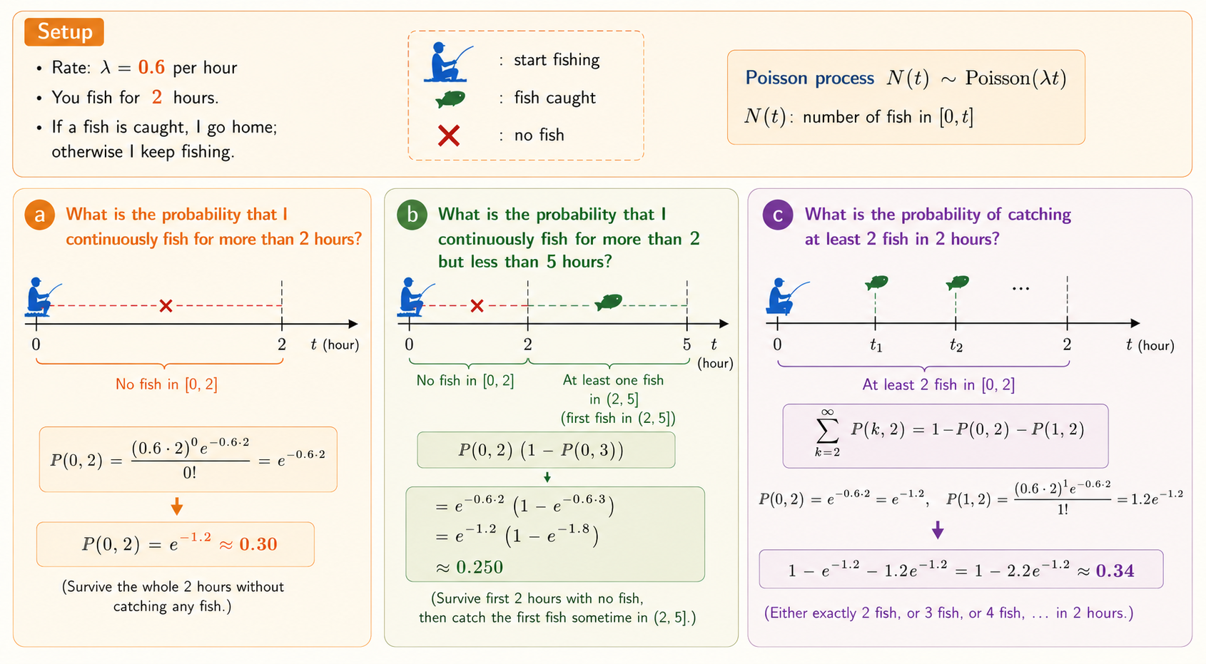
Suppose fish are caught according to a Poisson process with rate
\[ \lambda=0.6 \]
fish per hour. You always fish for two hours. If at least one fish is caught, you go home at time \(2\); otherwise, you continue until the first fish is caught.
Let \(N(t)\) denote the number of fish caught by time \(t\). Then
\[ N(t)\sim\operatorname{Poisson}(\lambda t), \]
and
\[ P(k,t)=\Pr(N(t)=k) = \frac{(\lambda t)^k e^{-\lambda t}}{k!}. \]
Fishing for More Than Two Hours
You continue beyond two hours exactly when no fish is caught during \([0,2]\):
\[ \Pr(T>2) = P(0,2) = e^{-0.6\cdot2} = e^{-1.2} \approx 0.301. \]
Fishing Between Two and Five Hours
This event requires no fish in the first two hours and at least one fish during the next three hours. Independent increments give
\[ \begin{aligned} \Pr(2<T<5) &=P(0,2)\bigl(1-P(0,3)\bigr)\\ &=e^{-1.2}\left(1-e^{-1.8}\right)\\ &\approx0.251. \end{aligned} \]
At Least Two Fish in Two Hours
Use the complement of zero or one arrival:
\[ \begin{aligned} \Pr(N(2)\ge2) &=1-P(0,2)-P(1,2)\\ &=1-e^{-1.2}-1.2e^{-1.2}\\ &\approx0.337. \end{aligned} \]
Expected Number of Fish
The expected number caught during the first two hours is
\[ E[N(2)]=\lambda\cdot2=1.2. \]
If no fish is caught by time \(2\), the policy guarantees exactly one additional fish before stopping. Therefore,
\[ \begin{aligned} E[N(T)] &=E[N(2)]+\Pr(N(2)=0)\\ &=1.2+e^{-1.2}\\ &\approx1.501. \end{aligned} \]
Expected Fishing Time
Starting from any time, the expected wait for the next fish is
\[ \frac{1}{\lambda}=\frac{1}{0.6}\approx1.667\text{ hours}. \]
The extra wait occurs only when no fish arrives in the first two hours. Hence
\[ \begin{aligned} E[T] &=2+P(0,2)\frac{1}{\lambda}\\ &=2+e^{-1.2}\frac{1}{0.6}\\ &\approx2.502\text{ hours}. \end{aligned} \]
Competing Exponentials: Light Bulbs
Install three light bulbs at the same time. Assume their independent lifetimes are
\[ X_1,X_2,X_3\sim\operatorname{Exponential}(\lambda). \]
We want the expected time until the last bulb burns out:
\[ E[\max(X_1,X_2,X_3)]. \]
Time Until the First Failure
The first failure is the minimum of three independent exponential clocks. Their rates add, so
\[ \min(X_1,X_2,X_3) \sim \operatorname{Exponential}(3\lambda), \]
with expected waiting time
\[ \frac{1}{3\lambda}. \]
After Each Failure
After the first bulb fails, two remain. By memorylessness, their residual lifetimes are again independent exponentials with rate \(\lambda\). The next failure therefore has expected additional wait
\[ \frac{1}{2\lambda}. \]
Once only one bulb remains, its expected additional lifetime is
\[ \frac{1}{\lambda}. \]
Thus,
\[ \begin{aligned} E[\max(X_1,X_2,X_3)] &=\frac{1}{3\lambda}+\frac{1}{2\lambda}+\frac{1}{\lambda}\\ &=\frac{11}{6\lambda}. \end{aligned} \]
The argument works because independent exponential clocks compete through the sum of their rates, while memorylessness resets the problem after each failure.
Bus Arrivals and Length Bias
Suppose bus interarrival times are equally likely to be five or ten minutes:
\[ \Pr(L=5)=\Pr(L=10)=\frac12. \]
If you arrive at a uniformly random time, you are more likely to land inside a long interval because it occupies more of the timeline.
Which Interval Do You Observe?
The observed interval has the length-biased distribution
\[ \Pr(L^*=\ell) = \frac{\ell\Pr(L=\ell)}{E[L]}. \]
Since \(E[L]=7.5\),
\[ \Pr(L^*=5) = \frac{5(1/2)}{7.5} = \frac13, \]
and
\[ \Pr(L^*=10)=\frac23. \]
Expected Wait to the Next Bus
Conditional on being inside an interval of length \(\ell\), a random observation point has expected residual wait \(\ell/2\). Therefore,
\[ \begin{aligned} E[W] &=\frac13\left(\frac52\right) +\frac23\left(\frac{10}{2}\right)\\ &=\frac{25}{6}\\ &\approx4.17\text{ minutes}. \end{aligned} \]
The value \(7.5\) minutes answers a different question: it is the expected next interval length if you arrive immediately after a bus departs. A random-time observer sees length bias and then arrives partway through the selected interval.
Key Takeaways
- Poisson counts and exponential waiting times describe the same arrival process from two perspectives.
- Independent increments make probabilities over consecutive time intervals easy to factor.
- Memorylessness lets a stopping problem restart after an arrival or failure.
- The minimum of independent exponential clocks is exponential with the sum of their rates.
- Sampling a process at a random time favors longer intervals, producing length bias.