19. Weak Law of Large Numbers
MIT 6.041SC Probabilistic Systems Analysis and Applied Probability
Notes on MIT 6.041SC Probabilistic Systems Analysis and Applied Probability, Lecture 19: Weak Law of Large Numbers, taught by John Tsitsiklis.
Suppose a pollster reports a sample fraction and promises to be within one percentage point of the population fraction with at least 95% probability. How many people must be sampled? Before choosing a number, we need to say what is random, what is fixed, and which sampling assumptions make such a promise meaningful. This first lecture in the course’s limit-theorems unit comes after the Markov-chain lectures.
The sample mean is random; the population mean is not
Let \(X_1,\ldots,X_n\) be independent, identically distributed (i.i.d.) measurements with finite mean \(\mu\) and variance \(\sigma^2\). The average from one sample is
\[ M_n=\frac{1}{n}\sum_{i=1}^n X_i. \]
The population mean \(\mu\) is a fixed number under this model. \(M_n\) is a random variable: another independently drawn sample can produce another average. Linearity of expectation and independence give two distinct facts:
\[ \mathbb E[M_n]=\mu, \qquad \operatorname{Var}(M_n) =\frac{1}{n^2}\sum_{i=1}^n\operatorname{Var}(X_i) =\frac{\sigma^2}{n}. \]
Unbiasedness alone says where the average of many hypothetical sample means would land. It does not promise that one sample mean is close. The \(1/n\) variance gives a route from that average statement to a probability bound for a single sample.
Chebyshev turns variance into a guarantee
For any random variable \(X\) with finite variance and any \(\varepsilon>0\), Chebyshev’s inequality says
\[ \Pr\bigl(|X-\mathbb E[X]|\ge\varepsilon\bigr) \le\frac{\operatorname{Var}(X)}{\varepsilon^2}. \]
It follows by applying Markov’s inequality to the nonnegative variable \((X-\mathbb E[X])^2\). This is a distribution-free bound: knowing the mean and variance is enough; knowing the full probability density is unnecessary. It may be loose. Applying it to \(M_n\) yields
\[ \boxed{\Pr\bigl(|M_n-\mu|\ge\varepsilon\bigr) \le\frac{\sigma^2}{n\varepsilon^2}.} \]
Fix any positive error tolerance \(\varepsilon\). As \(n\) grows, the right-hand side goes to zero. That proves the lecture’s version of the weak law of large numbers:
\[ M_n\xrightarrow{\Pr}\mu, \quad\text{meaning}\quad \forall\varepsilon>0,\ \Pr(|M_n-\mu|\ge\varepsilon)\longrightarrow 0. \]
“In probability” is doing real work here. It says the chance of landing outside any fixed band around \(\mu\) vanishes. It does not say every realized sequence of samples eventually stays inside the band. Nor does it supply a universal finite-sample accuracy without a variance and a sampling model.
A poll: 50,000 is a sufficient bound, not a forecast
Let \(X_i=1\) for “yes” and \(0\) for “no,” and let \(f\) be the true population yes-fraction. Under the lecture’s independent random-sampling model, \(\mathbb E[X_i]=f\) and \(\operatorname{Var}(X_i)=f(1-f)\le 1/4\). The sample mean \(M_n\) is the observed yes-fraction. For an error of at least one percentage point,
\[ \Pr(|M_n-f|\ge 0.01) \le\frac{f(1-f)}{n(0.01)^2} \le\frac{1}{4n(0.01)^2}. \]
To make this upper bound at most \(0.05\), it suffices to choose
\[ n\ge\frac{1}{4(0.05)(0.01)^2}=50{,}000. \]
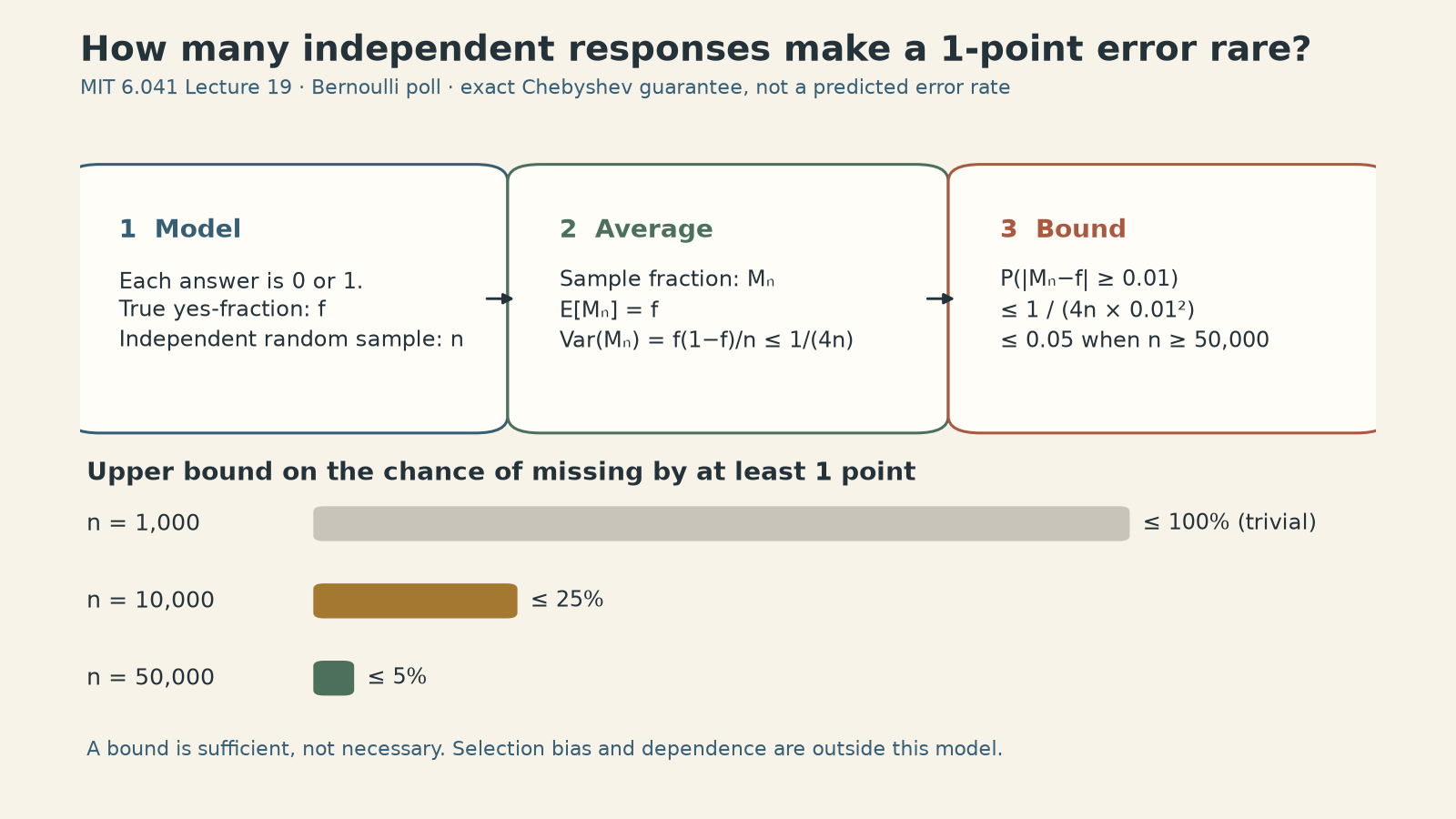
The figure shows a worst-case guarantee, not the actual error distribution. At \(n=1{,}000\), the raw Chebyshev expression is \(2.5\), so after the universal probability cap of \(1\) it says nothing useful. At \(n=50{,}000\), it certifies at most a 5% chance of missing by at least one point. The lecture calls this conservative and previews a sharper normal approximation in Lecture 20. We should not read “50,000” as the sample size every real poll needs.
More importantly, random-sampling assumptions are not cosmetic. A large convenience sample, systematic nonresponse, or dependent observations can miss the population fraction even when the arithmetic above is correct for the i.i.d. model. More samples reduce the model’s random variance; they do not automatically remove selection bias.
Why dependence changes the \(1/n\) story
As a constructed extension, suppose every measurement contains the same random disturbance \(Z\) plus its own independent noise \(E_i\): \(X_i=\mu+Z+E_i\), with \(\mathbb E[Z]=\mathbb E[E_i]=0\), \(\operatorname{Var}(Z)=\tau^2\), and \(\operatorname{Var}(E_i)=v\). Then
\[ M_n=\mu+Z+\frac1n\sum_{i=1}^n E_i, \qquad \operatorname{Var}(M_n)=\tau^2+\frac vn. \]
The independent noise fades; the shared disturbance does not. This is why simply replacing \(n\) in the lecture’s formula without checking dependence can create false precision.
A small tail probability can still carry a large expectation
The lecture gives a useful warning about the meaning of convergence in probability. Define \(Y_n=0\) with probability \(1-1/n\) and \(Y_n=n\) with probability \(1/n\). For every fixed \(\varepsilon>0\), once \(n\ge\varepsilon\),
\[ \Pr(|Y_n|\ge\varepsilon)=\frac1n\longrightarrow0. \]
So \(Y_n\) converges in probability to zero. Yet
\[ \mathbb E[Y_n]=n\cdot\frac1n=1, \qquad \mathbb E[Y_n^2]=n^2\cdot\frac1n=n. \]
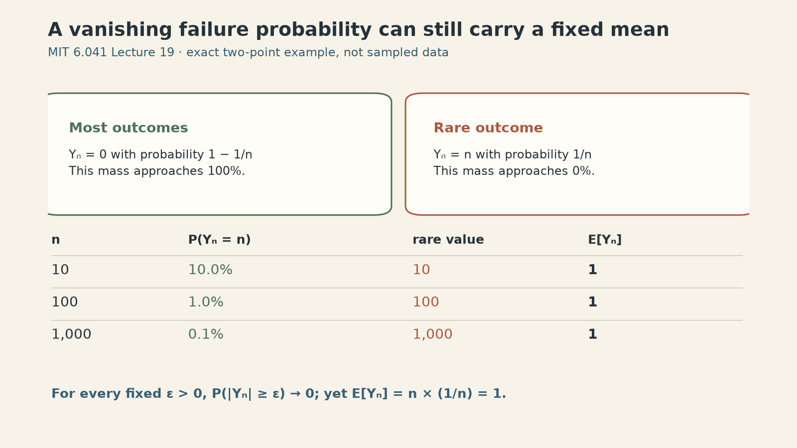
The increasingly unlikely event also becomes increasingly large. Convergence in probability controls the chance of being away from a target; by itself it does not control the size of the rare values or make expectations converge. This distinction matters when an “average case” hides a costly tail.
What the next limit theorem asks
The weak law answers whether \(M_n\) concentrates near \(\mu\). It does not describe the detailed shape of its residual fluctuations. Lecture 19 closes by comparing \(S_n=\sum_iX_i\), whose variance is \(n\sigma^2\), with \(M_n=S_n/n\), whose variance is \(\sigma^2/n\). To keep a nondegenerate scale, it introduces
\[ Z_n=\frac{S_n-n\mu}{\sigma\sqrt n} \quad(\sigma>0). \]
The central limit theorem concerns the distribution of \(Z_n\), not a claim that every finite-sample sum is exactly normal. That is the bridge to Lecture 20. For this lecture, the practical distinction is simpler: a sample average becomes reliable only relative to an error tolerance, a probability target, and assumptions one can defend.
Sources
- MIT OpenCourseWare, Lecture 19: Weak Law of Large Numbers (Fall 2013, John Tsitsiklis).
- Official Lecture 19 slides.
- Official Lecture 19 transcript.