20. Central Limit Theorem
MIT 6.041SC Probabilistic Systems Analysis and Applied Probability
Notes on MIT 6.041SC, Lecture 20: Central Limit Theorem, taught by John Tsitsiklis.
The weak law of large numbers says a sample average gets close to its population mean. The central limit theorem (CLT) asks a more detailed question: how likely is a particular error at a finite sample size? Its answer is a normal approximation—but only after centering and scaling the sum, and only under the theorem’s assumptions.
What converges to a normal distribution?
Let \(X_1,X_2,\ldots\) be independent and identically distributed (i.i.d.) from one fixed distribution with finite mean \(\mu\) and finite, positive variance \(\sigma^2\). Write \(S_n=\sum_{i=1}^n X_i\). The raw sum has mean \(n\mu\) and standard deviation \(\sigma\sqrt n\); both change with \(n\). We therefore study the centered and scaled sum
\[ Z_n=\frac{S_n-n\mu}{\sigma\sqrt n} =\frac{\sqrt n\,(M_n-\mu)}{\sigma}, \qquad M_n=\frac{S_n}{n}. \]
For every real number \(z\), the CLT says
\[ \Pr(Z_n\leq z)\longrightarrow\Phi(z), \]
where \(\Phi\) is the standard normal cumulative distribution function (CDF). It is the standardized sum’s CDF that converges. The theorem does not say the unscaled \(S_n\) settles into a fixed normal distribution, nor that a discrete sum suddenly has a continuous probability density.
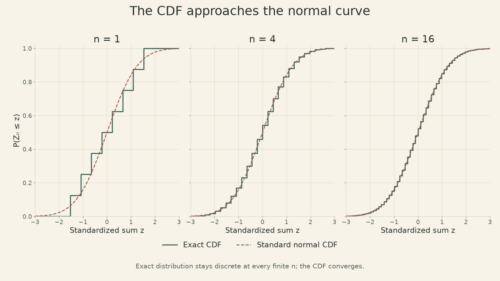
The figure uses exact convolution for independent fair draws from \(\{1,\ldots,8\}\), not a simulation. As \(n\) grows, the steps become smaller and the CDF follows the normal curve more closely. A strongly skewed starting distribution can converge less quickly at the same \(n\). The theorem gives a limiting result; it does not supply a universal sample size at which every normal approximation becomes accurate.
Revisiting the one-point poll
Suppose each independent, randomly sampled response is \(X_i\sim\mathrm{Bernoulli}(f)\), where the unknown population fraction is \(f\). The observed fraction \(M_n\) has mean \(f\) and variance \(f(1-f)/n\). Because \(f(1-f)\leq 1/4\), the standard deviation of \(M_n\) is at most \(1/(2\sqrt n)\).
We want the probability of an error of at least one percentage point to be no more than 5%. The earlier Chebyshev bound gives a sufficient, model-based guarantee:
\[ \Pr(|M_n-f|\geq 0.01) \leq\frac{f(1-f)}{n(0.01)^2} \leq\frac{2500}{n}. \]
So \(n=50{,}000\) makes that upper bound 0.05. The CLT instead estimates the two-sided tail by replacing the standardized fraction with a normal variable. Using the worst-case standard deviation \(1/2\), a 95% central normal interval has half-width approximately \(1.96/(2\sqrt n)\). Setting that to 0.01 gives
\[ n\approx\left(\frac{1.96}{2(0.01)}\right)^2\approx 9{,}604. \]
At \(n=10{,}000\), the same approximation gives \(2[1-\Phi(2)]\approx0.0455\) for the two-sided error probability. The contrast is useful: 50,000 is sufficient by a conservative inequality; about 9,604 is a normal-approximation planning number. The latter is not a rigorous 95% guarantee for every \(f\) and finite \(n\).
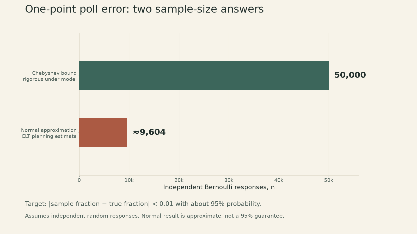
Both calculations depend on the sampling model. More responses reduce random sampling error; they do not remove selection bias or a shared disturbance among responses.
Why the cutoff moves by half a count
The lecture’s finite example is \(S\sim\mathrm{Binomial}(36,0.5)\), with mean 18 and standard deviation 3. Its exact cumulative probability through 21 is 0.8785:
\[ \begin{aligned} \Pr(S\leq21)&=\sum_{k=0}^{21}\binom{36}{k}2^{-36}\\ &\approx0.8785. \end{aligned} \]
A direct normal calculation at 21 uses \(\Phi((21-18)/3)=\Phi(1)\approx0.8413\) and misses the area represented by the integer-21 bar. To approximate a discrete event with a continuous curve, include the whole bar by moving its right edge to 21.5. That edge standardizes to \((21.5-18)/3=7/6\), so
\[ \begin{aligned} \Pr(S\leq21)&\approx\Phi(7/6)\\ &\approx0.8783. \end{aligned} \]
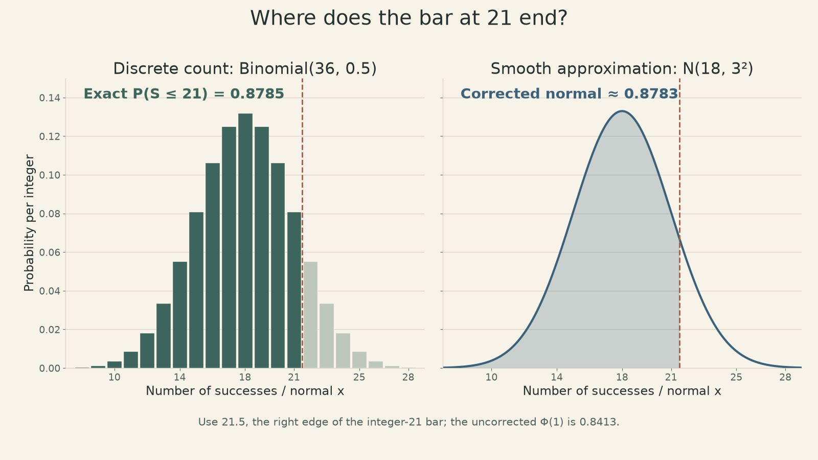
This continuity correction is a finite-sample approximation for integer counts. It does not change the CLT’s CDF statement. Its small error in this symmetric example should not be taken as a general accuracy promise for every binomial distribution.
Normal and Poisson are different binomial limits
For \(S_n\sim\mathrm{Binomial}(n,p)\) with a fixed \(0<p<1\), both its mean \(np\) and variance \(np(1-p)\) grow. Centering by \(np\) and dividing by \(\sqrt{np(1-p)}\) leads to the CLT’s standard normal limit. This is the regime behind the polling calculation.
Another regime lets \(p=p_n\) shrink as \(n\) grows while \(np_n\to\lambda\) remains finite. Then the count itself approaches a \(\mathrm{Poisson}(\lambda)\) distribution. The Bernoulli law changes with \(n\) here, so this is not a direct application of the fixed-law i.i.d. CLT. The approximation to choose depends on which quantities stay fixed: many moderately probable successes favor a normal description near the mean; rare events with a finite expected count favor Poisson.
The CLT is most valuable when its assumptions and scale are made visible. It can turn a bound into a sharper planning estimate, but a normal-looking curve never repairs a poor sampling design.
Source: MIT OCW Lecture 20 page · lecture slides · official transcript · video