22. Bayesian Statistical Inference II
MIT 6.041SC Probabilistic Systems Analysis and Applied Probability
Notes on MIT 6.041SC, Lecture 22: Bayesian Statistical Inference II, taught by John Tsitsiklis.
Can data have zero correlation with the quantity we want to estimate, yet determine it exactly? Yes. If \(X\) is uniform on \([-1,1]\) and \(\Theta=X^2\), knowing \(X\) reveals \(\Theta\), although \(\operatorname{Cov}(X,\Theta)=0\). A straight-line estimator misses that relationship.
This constructed example illustrates the distinction developed in Lecture 22: the best estimator under squared error and the best linear estimator solve different optimization problems. The previous lecture established the posterior mean as the squared-error optimum. This lecture studies its remaining uncertainty, its error properties, and what changes when the estimator must be a line.
A bounded measurement produces a nonlinear estimate
The lecture’s model has an unknown quantity and independent measurement noise:
\[ \begin{aligned} \Theta&\sim\operatorname{Uniform}(4,10),\\ U&\sim\operatorname{Uniform}(-1,1). \end{aligned} \] \[X=\Theta+U.\]
The joint density is \(1/12\) on the region \(4\leq\theta\leq10\) and \(|\theta-x|\leq1\), and zero elsewhere. For an observed \(3<x<11\), the possible values of \(\Theta\) form the interval
\[ \begin{aligned} A(x)&=\max(4,x-1),\\ B(x)&=\min(10,x+1). \end{aligned} \]
The joint density is constant along that interval, so the posterior is uniform on \([A(x),B(x)]\). Its mean is the midpoint:
\[ \begin{aligned} g_*(x)&=\mathbb E[\Theta\mid X=x]\\ &= \begin{cases} (x+5)/2,&3<x<5,\\ x,&5\leq x\leq9,\\ (x+9)/2,&9<x<11. \end{cases} \end{aligned} \]
In the middle, the entire noise interval is compatible with the prior, and the estimate equals the measurement. Near either end, the prior clips the interval and shifts its midpoint. The result has three straight segments but is not one affine function.
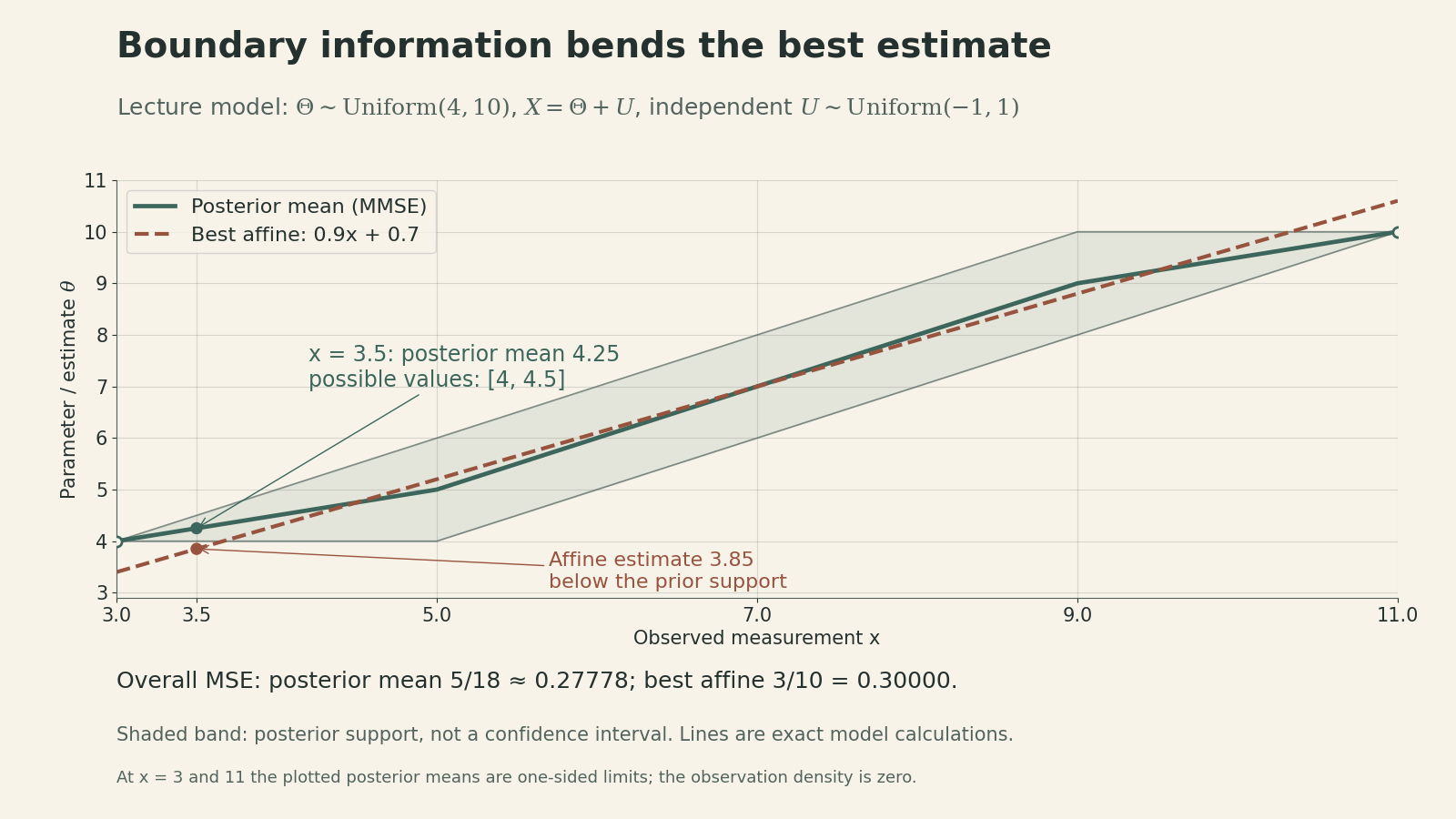
For example, \(x=3.5\) leaves only \(\Theta\in[4,4.5]\), so the estimate is \(4.25\). The observation falls below the prior’s lower bound because the noise can be negative; the unknown quantity itself still respects that bound.
Remaining uncertainty depends on the observation
Write \(L(x)=B(x)-A(x)\). The conditional squared-error risk of the posterior mean is the posterior variance:
\[ \begin{aligned} v(x)&=\operatorname{Var}(\Theta\mid X=x)\\ &=\frac{L(x)^2}{12}\\ &= \begin{cases} (x-3)^2/12,&3<x<5,\\ 1/3,&5\leq x\leq9,\\ (11-x)^2/12,&9<x<11. \end{cases} \end{aligned} \]
At \(x=3.5\), it is \(1/48\approx0.02083\). At \(x=7\), the posterior spans \([6,8]\) and the variance is \(1/3\). The same sensor can leave different amounts of uncertainty depending on the measurement.
The observation density is \(f_X(x)=L(x)/12\). It is zero at \(x=3\) and \(x=11\), so the density-ratio formula does not define the posterior there. The endpoint estimates \(4,10\) and variances \(0\) in the plots are one-sided limits.
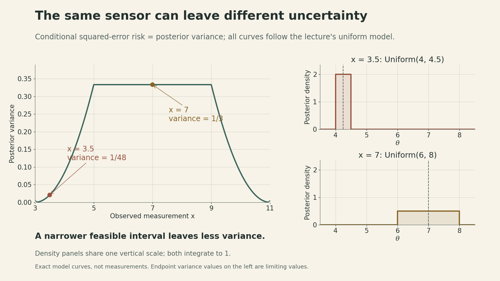
Averaging the posterior variance over measurements gives the overall minimum mean squared error:
\[ \begin{aligned} \operatorname{MMSE} &=\mathbb E[v(X)]\\ &=\int_3^{11}\frac{L(x)^3}{144}\,dx\\ &=\frac{5}{18}\approx0.27778. \end{aligned} \]
This value is an average over the model’s joint distribution, not the error on every realization.
Why the posterior-mean error is orthogonal to the data
Assume finite second moments. Let \(\hat\Theta=\mathbb E[\Theta\mid X]\) and \(e=\Theta-\hat\Theta\). Once \(X\) is given, \(\hat\Theta\) is known, so
\[ \begin{aligned} \mathbb E[e\mid X] &=\mathbb E[\Theta\mid X]-\hat\Theta\\ &=0. \end{aligned} \]
For any square-integrable function \(h(X)\),
\[ \begin{aligned} \mathbb E[e\,h(X)] &=\mathbb E\!\left[h(X)\mathbb E[e\mid X]\right]\\ &=0. \end{aligned} \]
In particular, the error has zero mean and is uncorrelated with the estimate. This is orthogonality, not independence: the conditional error variance can still depend on \(X\), as the bounded-noise example shows.
Zero mean here averages over the Bayesian joint model. It does not generally mean \(\mathbb E[\hat\Theta\mid\Theta=\theta]=\theta\) for every fixed parameter value, which is the usual classical unbiasedness requirement.
The same calculation gives the law of total variance:
\[ \begin{aligned} \operatorname{Var}(\Theta) &=\operatorname{Var}(\hat\Theta)\\ &\quad+\mathbb E[\operatorname{Var}(\Theta\mid X)]. \end{aligned} \]
The first term describes how the estimate varies as the data vary; the second is the uncertainty left after observing them. The expected remaining variance cannot exceed the prior variance, although this is not a pointwise guarantee for every observation in every model.
Orthogonality also explains why no other function of the same data can improve the mean squared error. Expanding the difference around \(\hat\Theta\) removes the cross term:
\[ \begin{aligned} \mathbb E[(\Theta-g(X))^2] &=\mathbb E[e^2]\\ &\quad+\mathbb E[(\hat\Theta-g(X))^2]. \end{aligned} \]
What restricting the estimator to a line buys
Computing a conditional mean can require difficult integrals. Linear least mean squares estimation instead chooses the best \(aX+b\). The name “linear” conventionally includes the intercept; mathematically this class is affine.
Let \(m_\Theta=\mathbb E[\Theta]\) and \(m_X=\mathbb E[X]\). Minimizing over the intercept gives \(b=m_\Theta-a\,m_X\). The remaining risk is
\[ \begin{aligned} R(a)&=\operatorname{Var}(\Theta)\\ &\quad-2a\,\operatorname{Cov}(X,\Theta)\\ &\quad+a^2\operatorname{Var}(X). \end{aligned} \]
For \(\operatorname{Var}(X)>0\), differentiating gives
\[ \begin{aligned} a_*&=\frac{\operatorname{Cov}(X,\Theta)} {\operatorname{Var}(X)},\\ \hat\Theta_L&=m_\Theta+a_*(X-m_X). \end{aligned} \]
Only means, variances, and covariance are needed. The measurement’s departure from its expected value corrects the prior mean; covariance sets the direction and size of that correction.
If both variances are positive, with correlation coefficient \(\rho\),
\[ \begin{aligned} R_L &=\operatorname{Var}(\Theta)\\ &\quad-\frac{\operatorname{Cov}(X,\Theta)^2} {\operatorname{Var}(X)}\\ &=\operatorname{Var}(\Theta)(1-\rho^2). \end{aligned} \]
It is the magnitude \(|\rho|\) that matters. At \(|\rho|=1\), an affine relation recovers the target almost surely. At \(\rho=0\), the best affine estimator is the prior mean; a nonlinear estimator may still learn much more. If \(X\) is constant, the slope formula is unavailable and the best prediction remains the prior mean.
For the bounded-noise model, \(\operatorname{Var}(\Theta)=3\), \(\operatorname{Var}(U)=1/3\), and \(\operatorname{Cov}(X,\Theta)=3\). Thus
\[ \begin{aligned} \hat\Theta_L&=7+\frac9{10}(X-7),\\ R_L&=\frac3{10}. \end{aligned} \]
The unrestricted risk is \(5/18\); the restriction adds \(1/45\approx0.02222\) in overall mean squared error. At \(x=3.5\), the affine estimate is \(3.85\), outside the prior support, while the posterior mean is \(4.25\). Optimality inside the affine class does not guarantee that every reported value is plausible under the full model.
Several measurements become a system of equations
For a scalar target and an \(n\)-dimensional observation vector, center the data and write
\[\hat\Theta_L=m_\Theta+a^\mathsf T(X-m_X).\]
Here \(a\) and \(m_X\) are \(n\)-vectors. Let \(\Sigma_X=\operatorname{Cov}(X,X)\) be an \(n\times n\) matrix and \(c=\operatorname{Cov}(X,\Theta)\) an \(n\)-vector. Differentiating the quadratic risk gives the normal equations
\[\Sigma_X a=c.\]
If \(\Sigma_X\) is invertible, the coefficients are unique. If it is singular, redundant features can make coefficients nonunique; solve within their span. A matrix of covariances is required, not just separate variances.
The lecture’s repeated-measurement model makes the weights particularly simple. Assume \(X_i=\Theta+W_i\), with mutually independent noises that are also independent of \(\Theta\), zero noise means, prior mean \(\mu\), and positive finite variances \(\tau^2=\operatorname{Var}(\Theta)\) and \(\sigma_i^2=\operatorname{Var}(W_i)\). Then
\[ \begin{aligned} \hat\Theta_L &=\frac{\mu/\tau^2+\sum_{i=1}^n X_i/\sigma_i^2} {1/\tau^2+\sum_{i=1}^n1/\sigma_i^2},\\ R_L&=\left(\frac1{\tau^2} +\sum_{i=1}^n\frac1{\sigma_i^2}\right)^{-1}. \end{aligned} \]
The prior mean acts like another weighted input. A noisy measurement receives less weight because its precision, the inverse variance, is smaller.
For a numerical extension, choose \(\mu=7\), \(\tau^2=3\), and observe \(X_1=6\), \(X_2=8\) with noise variances \(1\) and \(4\). The normalized weights on the prior and the two measurements are \(4/19\), \(12/19\), and \(3/19\). The estimate is \(124/19\approx6.5263\), with affine risk \(12/19\approx0.6316\).
These are LMMSE results without a Gaussian assumption. When the prior and the independent noises are Gaussian, the same estimate is also the posterior mean, and that risk is the posterior variance. Merely having normal-looking marginal distributions is not enough to assert a jointly Gaussian model.
“Linear” depends on the representation
The lecture compares observing \(X\) with observing \(X^3\). Cubing is invertible on the real line, so both observations contain the same information. The unrestricted conditional mean is unchanged after translating between the two representations. But the classes \(aX+b\) and \(aX^3+b\) differ.
The opening example makes this limitation exact. Take the constructed model \(X\sim\operatorname{Uniform}(-1,1)\) and \(\Theta=X^2\). Symmetry gives
\[ \begin{aligned} \operatorname{Cov}(X,\Theta)&=\mathbb E[X^3]=0,\\ \mathbb E[\Theta]&=1/3,\\ \operatorname{Var}(\Theta)&=1/5-1/9=4/45. \end{aligned} \]
The best affine function of \(X\) is therefore the constant \(1/3\), with risk \(4/45\). The unrestricted posterior mean is exactly \(X^2\), with zero risk. An estimator linear in the features \((X,X^2)\) can also recover \(\Theta\) exactly.
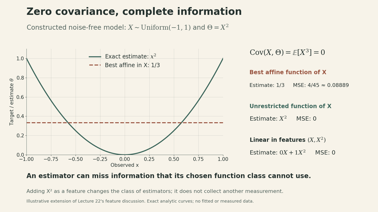
Feature construction enlarges the estimator class without adding a new measurement. The model determines what the data say; the loss determines what “best” means; the chosen function class determines which relationships the estimator can use. A formula for the best line should be read with all three choices in view.