A Stronger Statement Can Make the Proof Easier
Berkeley Advanced Large Language Model Agents · Lecture 11: Abstraction and Discovery with Large Language Model Agents
Why can proving a more general statement make a proof easier?
Suppose a compiler turns an arithmetic expression into stack-machine instructions. We want to show that the compiled program, starting from an empty stack, produces the expression’s value. That sounds like the simplest possible correctness claim. Yet it leaves out the context in which a subexpression actually runs: other values can already be on the stack, and more instructions can follow it.
The useful intermediate statement quantifies over those contexts. It says that compiling any expression has the same effect as pushing its value, for every initial stack and every continuation. This stronger contract lets the proofs of subexpressions compose.
That example is one thread in Swarat Chaudhuri’s Berkeley Lecture 11. The broader question is how an agent can discover reusable abstractions while searching. In mathematics, an abstraction can be a lemma that makes a proof possible. In empirical science, it can be a concept that guides the search for equations. Both require feedback, but the feedback establishes different things.
A proof assistant supplies a state, not just a verdict
The previous lecture studied plans, proof sketches, retrieved premises, and project context. Chaudhuri’s discussion of COPRA begins with the interaction that makes such reasoning checkable.
A proof state contains outstanding goals and the hypotheses available for each. A language model proposes a tactic; Lean or Coq executes it. The response can expose a new goal, report an error, or show that all obligations have been discharged. COPRA places relevant state, execution feedback, selected search history, and retrieved lemmas in the next prompt. Its search can backtrack when a branch is unproductive.
Learning here happens through changing context during a stateful search. It does not require updating model weights during that search. A failed tactic is also not a disproof of the theorem: it shows that this attempted move did not work. A timeout likewise leaves the problem unresolved.
The original COPRA paper evaluated particular models, proof environments, and query budgets in 2024. Its results support that feedback-and-search design in those settings; they are not a ranking of today’s models. A checker validates the proof of the formal statement. Whether that statement faithfully expresses the intended problem remains a separate question.
An informal plan can expose the right subgoals
The lecture’s number-theory example asks whether
\[\frac{21n+4}{14n+3}\]
is irreducible for every natural number \(n\). An informal solution suggests applying the Euclidean algorithm; the agent can turn the plan into smaller formal obligations, prove them, and use those proved lemmas in the final argument.
A compact arithmetic explanation is to write \(A=21n+4\) and \(B=14n+3\). Then
\[ \begin{aligned} 2A-3B &=2(21n+4)-3(14n+3)\\ &=-1. \end{aligned} \]
Every common divisor of \(A\) and \(B\) divides that integer linear combination, so their greatest common divisor is \(1\). The integer equation gives the reason the fraction is irreducible; a formal proof must also supply valid library facts and handle the representation of natural numbers and subtraction correctly.
An invented lemma name does not become usable because it appears in a plausible plan. The lecture shows how proof-environment feedback can reveal and repair that problem. The plan proposes a route; accepted subproofs justify the route.
Generalize the compiler theorem to its execution context
The compiler example uses natural-number constants, addition, and multiplication. Its source language is a recursive expression tree. Its target language is a list of instructions: push a constant, or apply a binary operator to the top two stack values. An instruction that needs two values fails if they are unavailable.
Let \(\mathrm{eval}(e)\) be the source expression’s value, \(\mathrm{compile}(e)\) its instruction list, and \(\mathrm{run}(p,s)\) the result of running program \(p\) on stack \(s\). The result is either a final stack or failure. Write \(v::s\) for pushing \(v\) on top of \(s\), and \(p\mathbin{\Vert}q\) for concatenating instruction lists.
The desired theorem is
\[ \begin{aligned} &\mathrm{run}(\mathrm{compile}(e),[\,])\\ &\qquad=\operatorname{Some}([\mathrm{eval}(e)]). \end{aligned} \]
Why is this statement awkward for induction? For a binary expression \(b(e_1,e_2)\), the lecture’s compiler emits the instructions for \(e_2\), then \(e_1\), then the operator \(b\). When \(e_1\) runs, the value of \(e_2\) is already on the stack. The empty-stack induction hypothesis does not directly describe that situation.
The auxiliary lemma supplies the missing context:
\[ \begin{aligned} &\forall e,p,s,\\ &\mathrm{run}(\mathrm{compile}(e)\mathbin{\Vert}p,s)\\ &\qquad=\mathrm{run}(p,\mathrm{eval}(e)::s). \end{aligned} \]
This is a statement about any whole expression, not merely a single machine instruction. The arbitrary continuation \(p\) describes what happens afterward; the arbitrary stack \(s\) describes what was already present. The equality also respects failure: if the continuation fails after consuming the pushed value, both sides have the same result.
![A constructed execution of the lecture's compiler evaluates (2+3) times 7. Starting with stack [11], the compiled instructions push 7, 3, and 2, then add and multiply, leaving [35,11]. A continuation that pushes 1 and adds produces [36,11]. The general lemma says that compiling the expression before this continuation is equivalent to pushing its evaluated value before the same continuation.](berkeley11-assets/stronger-compiler-lemma.png)
For a constant, the lemma follows from the push instruction. For a binary expression, let \(v_i=\mathrm{eval}(e_i)\). The induction hypothesis for \(e_2\) applies with the remaining code as its continuation. It leaves \(v_2::s\). The hypothesis for \(e_1\) then applies on that nonempty stack, leaving \(v_1::v_2::s\). Executing \(b\) gives \(b(v_1,v_2)::s\), which is exactly \(\mathrm{eval}(b(e_1,e_2))::s\); the arbitrary continuation now runs on that stack.
Setting both \(p\) and \(s\) to empty lists recovers the original theorem. More general is not automatically easier. Here it is easier to use because the generalized contract matches the recursive structure of the compiler.
The lecture presents the lemma as something an LLM can propose and COPRA can prove. Its value comes from both steps: invention makes the proof structure available, and verification makes the resulting abstraction safe to reuse under its stated assumptions.
LaSR searches for equations and concepts together
Scientific discovery has a different starting point: observations rather than axioms. Symbolic regression searches for a compact expression that explains a dataset. A candidate’s expression tree determines its structure, while parameters such as coefficients can be optimized numerically.
LaSR adds a learned library of natural-language concepts to evolutionary symbolic regression. A concept such as “periodic behavior” can connect expressions that differ syntactically. It can also guide proposals toward a relevant family of expressions.
The method alternates three phases:
- Hypothesis evolution: mix ordinary symbolic operations with concept-conditioned LLM proposals for initialization, mutation, and crossover. Evaluate candidates against data, accounting for expression complexity.
- Concept abstraction: describe patterns in promising expressions and contrast them with poor expressions. The paper uses candidates along the fit-versus-simplicity Pareto frontier as well as negative examples.
- Concept evolution: combine and extend concepts, then use the updated library to guide another round of expression search.
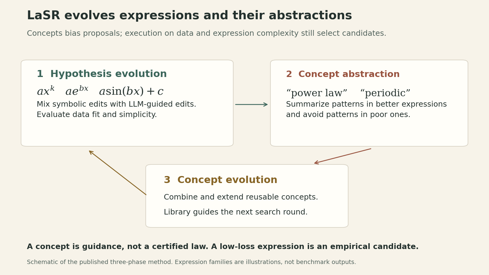
The paper frames this as a hierarchical model. Let \(D\) be the dataset, \(\pi\) an executable expression, and \(C\) a concept library. Its factorization is
\[ \begin{aligned} p(\pi,C\mid D) &\propto p(D\mid\pi)\\ &\quad\cdot p(\pi\mid C)\,p(C). \end{aligned} \]
The model assumes that the data depend on the expression, with concepts influencing the expression prior. Execution supplies evidence about data fit; the LLM supplies concept and expression proposals. This formulation does not mean that the implemented evolutionary search returns a calibrated posterior or an exact global optimum.
LaSR produces two artifacts: candidate equations and a reusable concept library. Yet the concepts themselves lack the proof assistant’s guarantee. In the published implementation, evolved concepts are added even when their correctness is difficult to quantify. A useful phrase can direct search; an appealing but wrong phrase can misdirect it.
A small residual is a different kind of evidence
Consider this constructed, noise-free dataset:
| \(x\) | \(y\) |
|---|---|
| 1 | 1 |
| 2 | \(1/4\) |
| 3 | \(1/9\) |
Both an inverse-square curve \(f(x)=1/x^2\) and the quadratic
\[ q(x)=\frac{11}{36}x^2-\frac53x+\frac{85}{36} \]
fit all three points exactly. At \(x=4\), however, \(f(4)=1/16\), while \(q(4)=7/12\). Their predictions differ by more than a factor of nine. If a new observation follows the constructed inverse-square model, it distinguishes these two candidates.
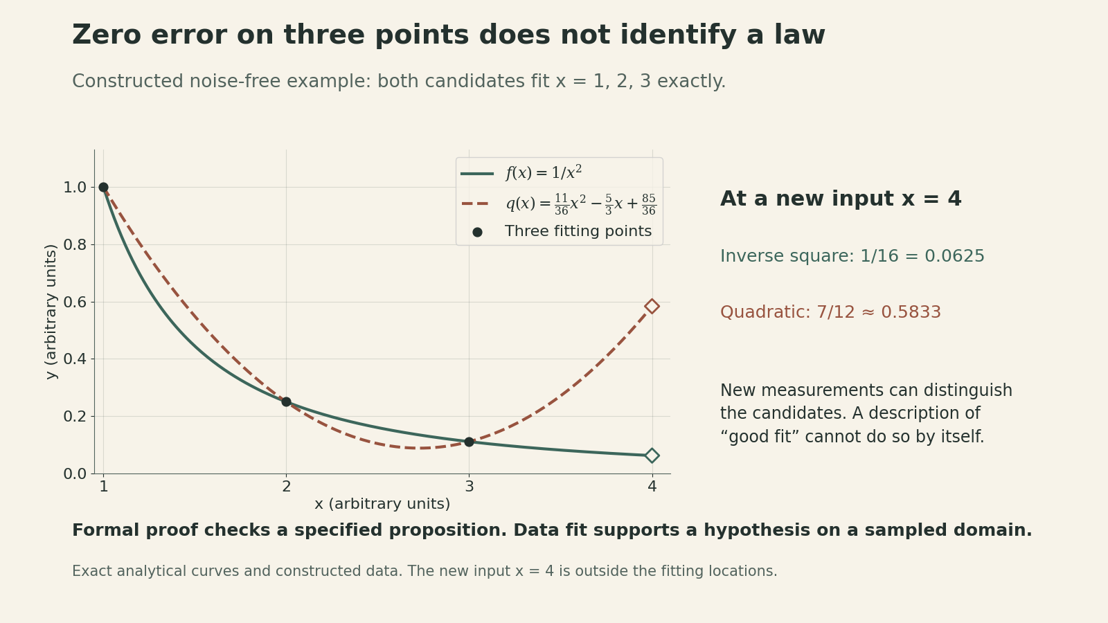
This is an illustration of the inference problem, not a LaSR experiment. A simplicity preference or domain knowledge can favor one candidate, but that preference is an assumption. Measurements in new regimes, dimensional constraints, and independent tests provide additional evidence.
The LaSR paper evaluates known physics equations and also generated synthetic equations to investigate whether gains depend on familiarity with famous laws. Those experiments address a specific leakage concern; they do not establish universal scientific validity. The paper also distinguishes exact symbolic recovery from thresholds on numerical error. Those are different success criteria.
Its BIG-Bench scaling-law case study is especially instructive. The authors search for an equation relating multiple-choice scores to training settings and the number of in-context examples, rather than fixing an equation skeleton in advance. Their appendix reports a generalization problem: the discovered relationship can behave differently for even versus odd numbers of examples, while the fitting data predominantly use odd counts. An interpretable equation makes that failure visible. It does not make the relationship a universal law of LLM behavior.
What transfers beyond mathematics
The slides also extend concept libraries to visual recognition. Descriptions such as a white head or a particular shape can become components of a visual decision program. A vision-language critic supplies a contrastive score to refine those descriptions. That score has the reliability of a learned evaluator, not the logical guarantee of a formal checker.
The remaining questions concern the representations and the evidence: which abstractions deserve reuse, how to express them beyond unconstrained language, how to search larger spaces, and how to choose informative experiments rather than only fit existing observations.
The connection I take from the lecture is a useful division of responsibilities. An LLM can suggest a generalization, a decomposition, or an equation family. A proof environment, execution engine, or new measurement must then establish what that suggestion supports. Reuse should preserve the assumptions and the kind of evidence attached to the abstraction.
Sources
- Berkeley Advanced Large Language Model Agents, Spring 2025 — course syllabus
- Swarat Chaudhuri — official Lecture 11 slides
- Official lecture recording
- Thakur et al. — An In-Context Learning Agent for Formal Theorem-Proving, COLM 2024
- Grayeli et al. — Symbolic Regression with a Learned Concept Library, NeurIPS 2024
- LaSR authors’ project page
- Curve values for the constructed fit example (CSV)