A Data Mixture Is Also a Repetition Schedule
Stanford CS336 Lecture 14: filtering, deduplication, mixing, and synthetic data
Giving half of a training budget to a small, carefully curated source can mean reading it fifty times. The sampling weight alone does not reveal that repetition. We also need the source size and the total number of training tokens.
Stanford CS336’s Spring 2026 Lecture 14, taught by Percy Liang, connects this problem to the rest of the data pipeline. Extraction determines what becomes text. Filtering determines which examples survive. Deduplication changes how often copied content appears. Mixing assigns training exposure, and synthetic-data generation creates new responses under a particular task and verification process.
The previous lecture followed data from its origin into a processed corpus. This lecture asks what happens between that corpus and the batches used for learning.
Extraction changes what the filter can see
An HTML page contains navigation, advertisements, content, and structure. Extracting its main text is not just deleting tags. Reading order, tables, code blocks, and headings affect what the resulting token sequence means. A nested table cannot always be flattened into prose without losing relationships.
The lecture contrasts fast rule-based HTML extraction with the additional work needed for PDFs. The FinePDFs example includes re-crawling truncated PDFs, extracting text with OCR or document-processing tools, and cleaning the result. PDF extraction can lose layout information, and the semantic structure supplied by HTML tags such as headings and paragraphs is not necessarily preserved.
This matters downstream: a quality classifier scores the extracted representation. If extraction duplicates a footer or scrambles a table, a later filter sees that artifact. A document’s original value and the usefulness of its extracted text can differ.
A quality score inherits its target
The lecture frames filtering as finding examples in a large raw pool that resemble a smaller target collection. The target supplies an operational meaning of quality: mathematical writing, instructional code, a particular language, or a desired style of discourse.
Two common approaches implement this idea differently. A language model fitted to the target can score how predictable a document is under that distribution. For variable-length documents, average log-likelihood or perplexity avoids comparing raw sequence probabilities as if length did not matter. A classifier instead distinguishes target examples from background data and applies its learned score to the large pool.
The classifier’s output is evidence about its training labels. It is not an independent measurement of factual truth or universal educational value. The positive examples, negatives, features, and threshold all influence what survives.
The lecture’s examples show several ways to specify a target:
- Language identification: fastText models classify language, with practical complications from mixed-language text and dialects.
- Mathematical text: OpenWebMath combines indicators such as LaTeX, a target language model, and a classifier rather than relying on one universal score.
- Educational code: the phi-1 example uses an expensive model to label a sample, then trains a cheaper classifier to select from a larger code pool. That classifier uses embeddings produced by a pretrained CodeGen model.
- Toxicity filtering: the labels come from annotated discourse, so the meaning of a rejection depends on that annotation task and its transfer to new text.
A stricter threshold usually trades quantity for closer resemblance to the target. Whether that trade helps depends on the training budget. A small selected corpus may work well early and become heavily repeated later. The lecture illustrates this with a finite-pool training comparison; it does not establish one threshold that is best at every scale.
The coupling is simple. Tightening a filter reduces the available source size. If its sampling share and the total training budget remain fixed, its equivalent number of passes rises. Filtering and mixing therefore cannot be optimized independently of repetition.
Deduplication needs a definition of the repeated item
A mirrored page, a forked repository, and a paragraph reused inside otherwise different documents are different kinds of duplication. Before choosing an algorithm, three decisions are needed: the unit being compared, the similarity rule, and the action taken after a match.
Document-level exact matching keeps one copy of an identical document. Span-level matching can remove repeated passages inside different documents, but deleting a middle passage may damage coherence. Near-duplicate detection admits changes such as formatting or a few substituted words. The chosen granularity determines which information the procedure can remove.
The deduplication study by Lee and colleagues reports benefits for efficiency and reduced memorization in its experiments. Deduplication is not a complete privacy guarantee. It also differs from decontamination, which explicitly checks overlap between training material and protected evaluation data. Deduplicating each source separately does not remove duplicates shared across sources.
Hash equality is not string equality
The lecture’s exact-deduplication demonstration groups strings by a MurmurHash value and keeps one item per group. It is a compact illustration, but two different strings can have the same finite hash. If exact equality is the requirement, hash groups need an equality check before distinct strings are discarded.
The demonstration also sorts items before grouping. That sorting step takes comparison-based \(O(N\log N)\) time for \(N\) items; the example is not a proof that every deduplication pipeline runs in linear time. Hash partitioning can avoid all-pairs comparisons, while skewed buckets, signature computation, communication, and candidate verification still contribute to the cost.
MinHash turns set overlap into a probability
To compare documents approximately, represent each as a set of features, often short consecutive token sequences called shingles. The shingle length and normalization policy are part of the definition. Using a set discards feature multiplicity, and it preserves only the local ordering encoded inside each shingle.
For nonempty sets \(A\) and \(B\), their Jaccard similarity is
\[ s=J(A,B)=\frac{|A\cap B|}{|A\cup B|}. \]
The lecture uses \(A=\{1,2,3,4\}\) and \(B=\{1,2,3,5\}\), giving \(s=3/5=0.6\).
Imagine drawing a uniformly random permutation of the feature universe and recording the first member of each set. Those two minima agree exactly when the first element of \(A\cup B\) belongs to \(A\cap B\). Each union element is equally likely to be first, so
\[ \Pr[h_{\min}(A)=h_{\min}(B)]=J(A,B). \]
This identity is exact under the ideal random-permutation construction. Practical implementations approximate it with seeded finite hash functions; collisions and departures from the ideal family need to be considered separately.
With \(m\) independent ideal signatures, the fraction of matching signatures estimates \(s\). Its standard deviation is
\[ \sqrt{\frac{s(1-s)}{m}}. \]
For \(s=0.6\) and \(m=100\), that is about \(0.049\). A particular set of seeds can happen to give exactly \(0.6\); a hundred signatures do not guarantee an error smaller than \(0.01\). Most importantly, one matching signature does not prove that the similarity exceeds a chosen threshold.
LSH generates candidates; verification decides what to remove
MinHash locality-sensitive hashing groups \(m=br\) signatures into \(b\) bands with \(r\) rows each. A pair becomes a candidate if, in at least one band, all \(r\) rows match.
Under the independent ideal-signature model, a fixed band matches with probability \(s^r\). No band matches with probability \((1-s^r)^b\). Therefore,
\[ P_{\mathrm{candidate}}(s)=1-(1-s^r)^b. \]
For the lecture’s worked configuration \(s=0.8\), \(b=5\), and \(r=10\), the candidate probability is about \(0.433\). This is a probability of being retrieved for comparison, not a posterior probability that the documents are duplicates.
At fixed \(b\), more rows per band make matches harder. At fixed \(r\), more bands give more chances to match. Both changes also alter the total signature count unless another parameter is adjusted. The figure starts from ten bands and ten rows, then changes one parameter at a time.
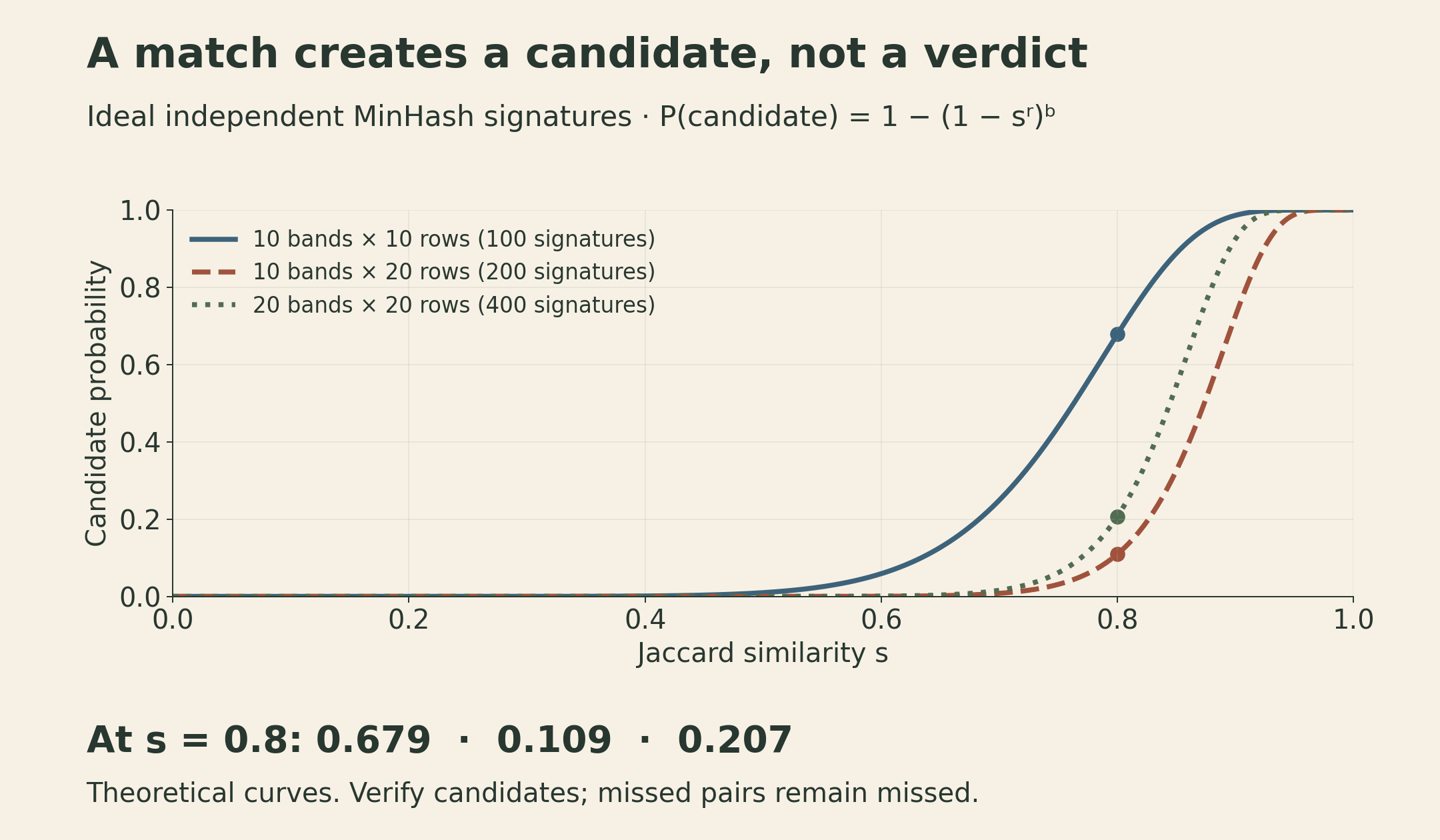
The often-used scale \(s_*=(1/b)^{1/r}\) is not an exact cutoff. At that similarity,
\[ P_{\mathrm{candidate}}(s_*)=1-(1-1/b)^b, \]
which approaches \(1-e^{-1}\approx0.632\) for large \(b\). Pairs below it can still be retrieved; pairs above it can still be missed.
A subsequent similarity check can reject false candidates. Lee and colleagues, for example, combine MinHash candidate selection with an edit-similarity check. Their paper uses the opposite symbols for bands and rows; the probability formula here follows the definitions above. Such verification cannot recover a pair that candidate generation never retrieved. The retained representative and any clustering policy are additional choices: a chain of pairwise matches need not mean every pair in a cluster exceeds the same threshold.
A source weight implies an exposure budget
Let \(D\) be the total training-token budget, \(p_i\) the fraction allocated to source \(i\), and \(N_i\) its available tokens under one fixed tokenizer. Define equivalent passes as
\[ e_i=\frac{p_iD}{N_i},\qquad \sum_i p_i=1. \]
Here \(p_i\) denotes a token share, or an equal-length training-sequence share that induces the same token share. A probability over variable-length documents is not automatically equivalent. Under stochastic sampling, these are expected allocations rather than a promise that every example is visited equally often.
Use the lecture’s illustrative two-source setting: an abundant pool of 10 trillion tokens, a scarce curated pool of 10 billion tokens, and a training budget of 1 trillion tokens. A 50/50 allocation gives each pool 500 billion training tokens. That is \(0.05\) equivalent passes over the abundant source and \(50\) over the scarce one.
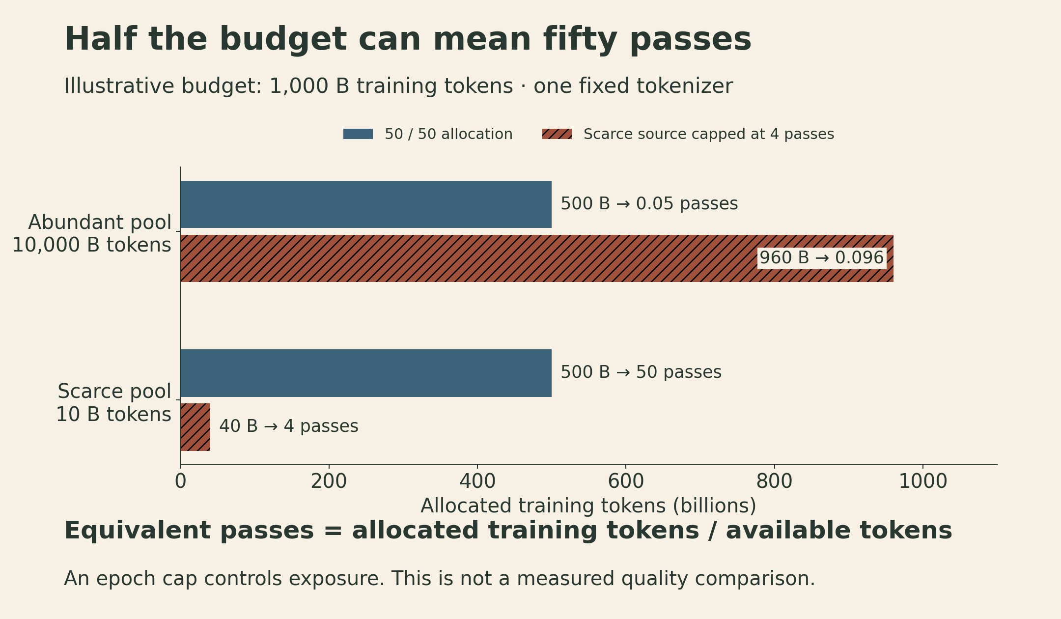
Repetition is not automatically useless: a second pass can still improve a model. But the 50/50 label hides a large difference in exposure, and additional passes can eventually bring diminishing returns or overfitting. The formula reveals the repeated exposure; it does not predict the loss curve.
An epoch cap must include source size
UniMax balances language allocations as uniformly as possible while limiting repetitions of each language’s corpus. The original algorithm expresses both the budget and the corpus sizes in characters; it denotes the budget by \(C\) and the epoch limit by \(N\). In the token-count formulation here, we instead use \(C\) for the epoch cap:
\[ \frac{p_iD}{N_i}\le C \quad\Longleftrightarrow\quad p_iD\le C N_i. \]
The right side must have units of tokens. Writing only \(p_iD\le C\) would be wrong when \(C\) counts epochs.
For a constructed cap of four passes, the 10-billion-token source can supply at most 40 billion training tokens. Its share of the 1-trillion-token run is therefore at most \(0.04\). Allocating the remaining 960 billion tokens to the large source gives \(0.096\) passes there.
This illustrates UniMax’s allocation principle: cap a source whose uniform allocation would exceed its capacity, then distribute the remaining budget across the other sources. A feasible full allocation requires enough total capped capacity, \(D\le C\sum_iN_i\). The cap controls repetition; it does not prove that the resulting mixture is best for the intended tasks.
A small proxy run should reproduce the relevant scarcity
Regression-based mixing methods train small models on several candidate mixtures, fit a predictor from mixture weights to an evaluation objective, and optimize that predictor before choosing a larger run’s mixture. The lecture discusses RegMix and Olmix within this framework.
Two different transfers must work. The predictor must remain reliable near the mixture selected by optimization, which may lie far from well-sampled regions. And the ranking of mixtures must transfer from small runs to the intended model and training budget. Repeated tuning on a narrow evaluation suite can also favor that suite rather than broad capability.
Finite data creates one predictable mismatch. A 10-billion-token proxy run can allocate half its budget to a 10-billion-token source without even finishing one pass. A 1-trillion-token run with the same weights makes fifty passes over that source.
Simulated epoching addresses this mismatch by downsampling each source in proportion to the reduction in training budget. Let \(D_s\) and \(D_L\) be the small and large budgets, and use
\[ N_i^{(s)}=N_i^{(L)}\frac{D_s}{D_L}. \]
Then, for the same weights,
\[ \frac{p_iD_s}{N_i^{(s)}} =\frac{p_iD_L}{N_i^{(L)}}. \]
With \(D_s=10\) billion and \(D_L=1000\) billion, source pools are reduced by a factor of 100. The scarce pool becomes 0.1 billion tokens. A 50% share gives it 5 billion training tokens, again producing fifty equivalent passes.
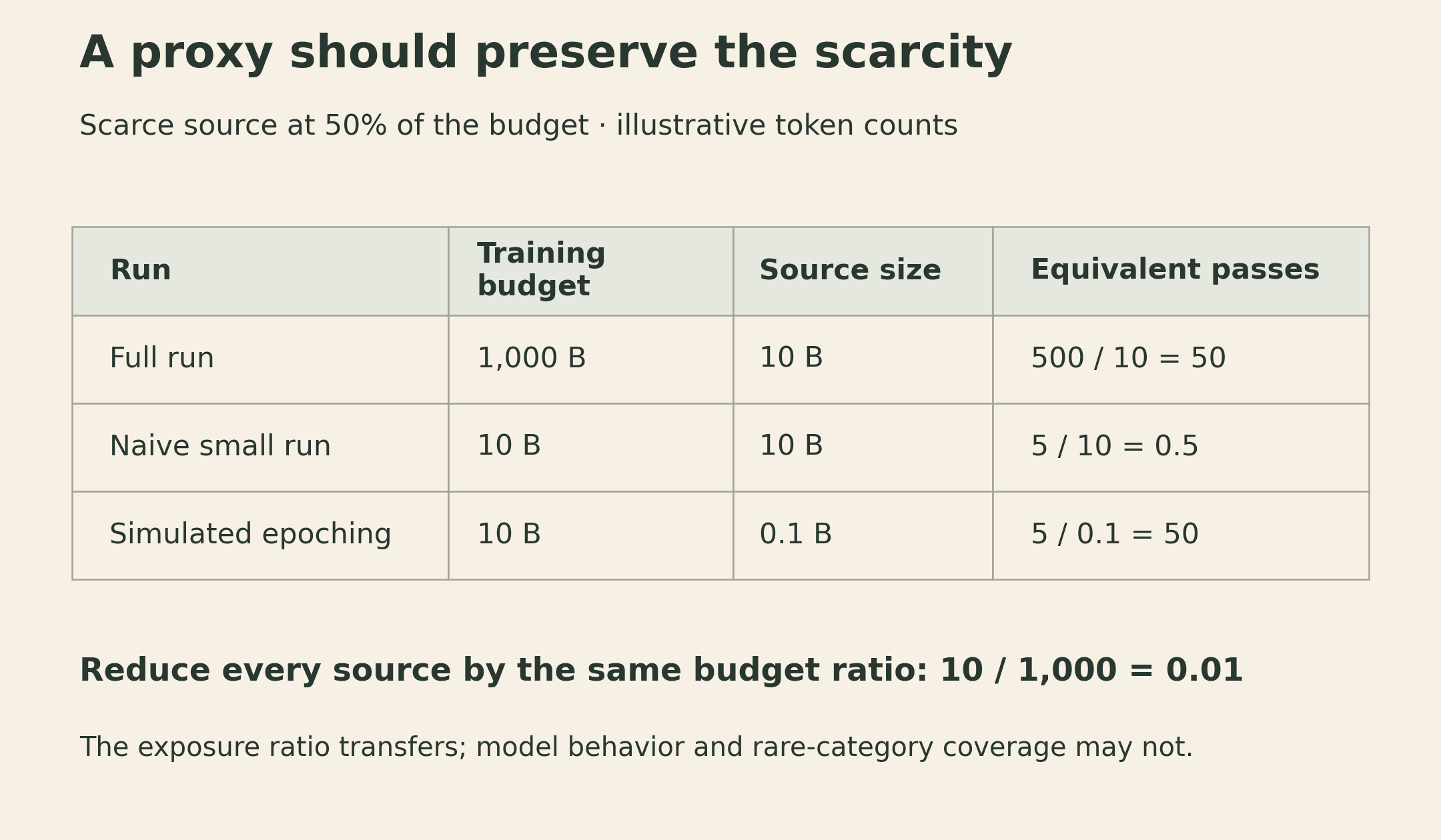
The UtiliMax paper describes this subsampling construction for simulating data constraints. It preserves the exposure ratio, not every property of large-scale training. Downsampling can lose rare categories, and very small sources create rounding and coverage problems. Model capacity, optimization, and the evaluation objective still matter.
Synthetic data adds a teacher and a verification process
For post-training, the unit is often a question–response pair or a complete agent trajectory. The lecture separates three ingredients: the environment, the task or prompt, and the response produced by a teacher. Counting generated responses does not count distinct tasks.
OpenThoughts studies these choices through reasoning-data experiments. For code and science, its combinations of question deduplication and multiple answers yield similar results. For math, exact deduplication with four answers per question performs best; sixteen answers is second-best and is adopted partly for scalability. On the reported benchmark averages, its answer-filtering variants do not beat the unfiltered baseline, but that baseline trains on 63,200 pairs rather than the filtered variants’ 31,600, so this is not a compute-controlled comparison. Among the equal-size math subsets, random subsampling beats the other filtering methods. The reported benchmark averages also favor responses generated by QwQ-32B over those from DeepSeek-R1 as student-training data, despite the latter’s stronger scores on several evaluations. Those results concern the student, data, and training recipe studied, not a general ranking of teachers or a reason to stop checking correctness.
For software engineering, the environment adds another constraint. The lecture surveys SWE-smith, which constructs repair tasks by modifying real repositories, and SWE-rebench, which mines pull requests and builds task environments. It also discusses a separate dataset release, SWE-ZERO-12M-trajectories, that scales the SWE-Zero setup across executable and non-executable tasks. Repository availability, number of tasks, number of sampled trajectories, and successfully verified repairs are separate quantities.
SWE-Zero to SWE-Hero makes the distinction especially clear. The SWE-Zero phase collects repository-editing trajectories in a generic sandbox without code execution. Its filtering rejects prohibited execution attempts, malformed trajectories, and edits to files present in the test patch. The SWE-Hero phase uses a smaller set with execution feedback. Removing future repository history addresses a specific shortcut; it does not certify every generated patch or every aspect of an agent’s behavior.
An execution-free trace can be useful training material without constituting a tested repair. Passing tests, where available, establishes a result only under those tests. Neither that result nor successful task completion is a general safety or authorization check.
The connection back to pre-training is the allocation of evidence and exposure. A filter selects a proxy for usefulness. LSH selects candidate overlaps. A mixing policy allocates repeated observations. A teacher generates possible responses. Each step changes what the student learns from, and each has a different way to be wrong.
Lecture and further reading
- Stanford CS336 Spring 2026, Lecture 14, Percy Liang: transformation, filtering, deduplication, mixing, and synthetic data.
- Pinned lecture code.
- Mining of Massive Datasets, Chapter 3: shingling, MinHash, and locality-sensitive hashing.
- Lee et al., Deduplicating Training Data Makes Language Models Better.
- Chung et al., UniMax, Section 3 and Algorithm 1.
- Optimizing Pretraining Data Mixtures with LLM-Estimated Utility, data-constrained experiments.
- Data Recipes for Reasoning Models, Sections 4.4–4.6.
- From SWE-Zero to SWE-Hero, trajectory collection and filtering.