What Biobank Associations Can Tell Us—and What They Cannot
MIT 6.874 Spring 2021 · Lecture 14: Systems Genetics and Electronic Health Records
A biobank can connect genetic variants to thousands of measurements, diagnoses, and questionnaire responses. That scale changes the questions we can ask. Instead of following one significant variant, we can estimate how genetic signal is distributed across the genome, identify patterns shared by many traits, and build predictors from many small effects.
Those are three different tasks. Explaining variation across a population, organizing association patterns, and predicting an individual’s phenotype require different evidence. A useful result for one task does not automatically solve the others.
MIT 6.874 Lecture 14, taught by Manolis Kellis with guest lectures from Alkes Price and Manuel Rivas, follows these connections. Price explains how LD Score regression uses correlated variants to study heritability and relevant cell types. Rivas turns to biobanks that combine genetics with electronic health records, questionnaires, biomarkers, and imaging, then shows how association matrices and polygenic predictors summarize that information.
Heritability is a population quantity, not an individual verdict
Under a decomposition \(Y=A+E\), where \(A\) is the additive genetic component and \(E\) collects the remaining variation, assume \(\operatorname{Cov}(A,E)=0\). Narrow-sense heritability is
\[ h^2=\frac{\operatorname{Var}(A)}{\operatorname{Var}(Y)}. \]
The population and environment are part of that definition. It is not the fraction of one person’s outcome that was “caused by genes,” and a large value does not imply that changing the environment is ineffective. Broad-sense heritability includes non-additive genetic variation as well.
Price starts his guest lecture with a useful definition of SNP heritability for a specified set of variants: the best population-level squared correlation between the phenotype and a linear combination of their genotypes. That target differs from the test-set performance of a predictor learned from a finite dataset. It also depends on which variants are included and how well they tag relevant variation. For binary outcomes, observed-scale and liability-scale estimates additionally depend on their definitions and sampling assumptions; they are not interchangeable percentages.
For fixed effects \(\mathbf b\) and a random individual’s standardized genotype vector \(\mathbf x\) with population correlation matrix \(R\),
\[ \operatorname{Var}(\mathbf x^\top\mathbf b)=\mathbf b^\top R\mathbf b. \]
One cannot generally replace this expression by \(\sum_j b_j^2\) when variants are correlated. In the random-effects model used below, mean-zero independent effects make the cross terms vanish in expectation over effects. That is an assumption of the model, not a statement that LD is absent.
A simple calculation also separates effect size from variance explained. For an allele dosage \(G\sim\operatorname{Binomial}(2,f)\) under Hardy–Weinberg equilibrium, a per-allele effect \(b\) contributes
\[ \operatorname{Var}(bG)=2f(1-f)b^2. \]
In a constructed example, \(f=0.5,b=0.1\) gives \(0.005\) phenotype-units squared. With \(f=0.01,b=0.3\), the contribution is \(0.001782\). The rarer allele has three times the per-allele effect but less variance in this population. These numbers are variance contributions, not heritability fractions unless divided by the relevant total phenotypic variance.
The “missing heritability” discussion asks why genome-wide significant loci explain less variation than broader genetic estimates. Many small effects below the significance threshold, poorly tagged variants, and model assumptions can all matter. It does not follow that there is one missing biological mechanism waiting to be found.
Annotation enrichment must account for neighboring variants
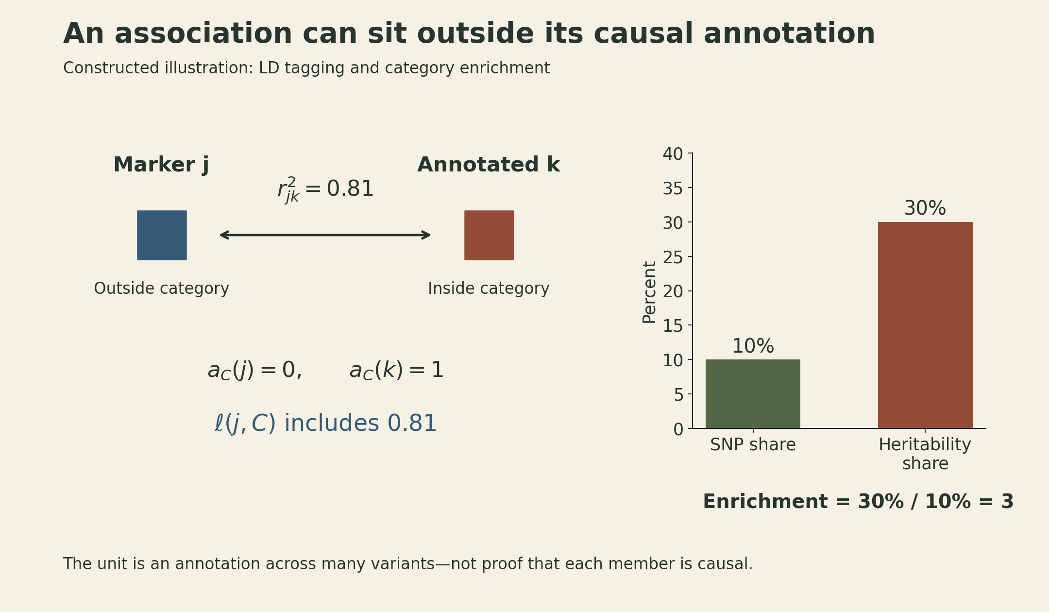
Suppose we want to know whether variants in an enhancer annotation contribute unusually strongly to a trait. Comparing the association statistics of enhancer SNPs with all other SNPs is inadequate. A SNP outside the annotation can have a strong statistic because it tags a SNP inside it.
For annotation \(c\), let \(a_c(k)\) equal one when variant \(k\) belongs to that annotation and zero otherwise. Define
\[ \ell(j,c)=\sum_k r_{jk}^2a_c(k), \qquad \operatorname{Var}(b_k)=\sum_c\tau_c a_c(k). \]
Then the stratified model is
\[ \mathbb E[\chi_j^2] \approx 1+c_0+N\sum_c\tau_c\ell(j,c). \]
Here \(c_0\) denotes intercept inflation; it is not an annotation index. Multiple regression estimates the annotation coefficients \(\tau_c\). If annotations overlap, an individual coefficient is a conditional contribution to per-SNP effect variance, not the complete heritability of that category. The model-derived category contribution sums the fitted per-SNP variances over its members:
\[ H_C=\sum_{k\in C}\sum_c\tau_c a_c(k), \qquad \operatorname{Enrichment}(C)=\frac{H_C/H_{\mathrm{all}}}{|C|/M}. \]
Here \(H_{\mathrm{all}}\) sums the fitted per-SNP variances over all \(M\) modeled variants. Overlapping category contributions need not sum to the total, because a variant can appear in several categories. A category containing 10% of variants and accounting for 30% of modeled SNP heritability has threefold enrichment. It does not follow that every variant in it is causal.
Price’s examples connect regulatory annotations to biologically plausible tissues, such as brain annotations for schizophrenia and immune annotations for rheumatoid arthritis. Those are aggregate statistical results. They do not identify the causal nucleotide at each locus or establish that one cell type is the only relevant tissue.
The baseline annotation model matters. At roughly 36–41 minutes, Price shows why omitted categories can bias estimates and why a richer baseline can reduce that problem in the examined simulations. He also warns about annotations built from the top cis-eQTL at each locus: those selected tags need not satisfy the assumed effect-variance model. A functional-sounding label does not make an annotation statistically valid. Finucane et al. give the model and its uncertainty procedure.
Biobanks turn many associations into a matrix
Rivas shifts from one trait to many. A variant can associate with several phenotypes, while a phenotype can associate with many variants. The resulting many-to-many relationship is difficult to interpret as thousands of separate plots.
DeGAs—Decomposition of Genetic Associations—applies truncated singular value decomposition to a prepared association matrix. Let \(W\) have \(T\) phenotype rows and \(M\) variant columns. Its rank-\(K\) approximation is
\[ W\approx U_KS_KV_K^\top, \qquad U_K\in\mathbb R^{T\times K},\quad S_K\in\mathbb R^{K\times K},\quad V_K\in\mathbb R^{M\times K}. \]
A column of \(U_K\) describes phenotype loadings; a column of \(V_K\) describes variant loadings. Singular values scale their contributions. This is a decomposition of genetic association summaries, not PCA of individual patients’ raw electronic records.
The published Tanigawa et al. study analyzed 2,138 phenotypes in its all-non-MHC dataset. Its final matrix included 235,907 variants after quality control and LD pruning, exclusion of the MHC, and association-value filtering. The methods specify \(p<0.001\) and standard-error filters, followed by within-phenotype centering and scaling. These choices define the matrix being decomposed; it is not an unfiltered table of every association in the biobank.
To illustrate the factorization alone, use a small matrix that is not standardized as in DeGAs:
\[ W=\begin{bmatrix} 2&2&0\\ 1&1&0\\ 0&0&3 \end{bmatrix} =\sqrt{10}\,\mathbf u_1\mathbf v_1^\top +3\,\mathbf u_2\mathbf v_2^\top, \]
with \(\mathbf u_1=(2,1,0)^\top/\sqrt5\), \(\mathbf v_1=(1,1,0)^\top/\sqrt2\), and \(\mathbf u_2=\mathbf v_2=(0,0,1)^\top\). Its two nonzero singular values are \(\sqrt{10}\) and \(3\). The leading component captures \(10/19\approx52.6\%\) of the matrix’s squared Frobenius norm; the second captures \(9/19\approx47.4\%\). Keeping only the first would discard the pattern carried by the third trait and third variant. This toy matrix illustrates the factorization only; it is not the study’s preprocessing output or empirical data.
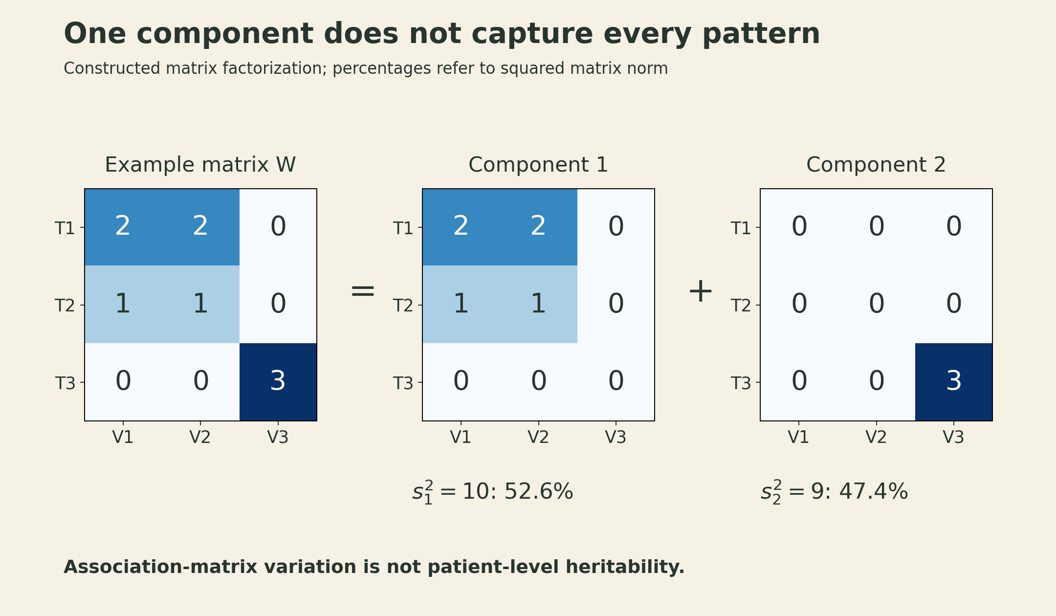
This distinction about the denominator is essential. A component’s share of association-matrix variation is not the fraction of patient-level phenotypic variance it explains. The component sign is also arbitrary: flipping both singular vectors leaves their product unchanged. Orthogonal mathematical components are not necessarily independent biological pathways.
In the lecture, body-mass associations separate into components related to fat and fat-free mass. The study uses those patterns to prioritize variants and genes, then adds functional follow-up in adipocyte models. The experimental evidence is an additional step; a loading or a compelling label alone does not establish mechanism.
A protective association can expose a tradeoff
The EHR and biobank setting supplies many measured outcomes for the same genetic variation. That can help reveal both potential benefit and possible harm. Rivas discusses predicted protein-truncating variants as clues to gene function and therapeutic hypotheses, including an IFIH1 example with favorable associations for some autoimmune phenotypes but an unfavorable association for ulcerative colitis.
The inference is narrower than “turn off this gene to treat disease.” A predicted truncating variant may affect particular transcripts; lifelong genetic exposure is not identical to a drug administered at a chosen dose and age. Observational associations and experimental follow-up can motivate a target hypothesis without establishing clinical efficacy or safety.
Similarly, the data source must remain visible. Electronic health records, questionnaires, laboratory measurements, and imaging do not define interchangeable phenotypes. Combining summaries across biobanks requires compatible phenotype definitions, allele alignment, and a suitable statistical model. More rows in a matrix cannot repair a mismatched outcome definition.
Prediction needs its own objective and its own test population
A polygenic score is a weighted genotype sum,
\[ \operatorname{PGS}_i=\sum_j w_jg_{ij}. \]
Marginal GWAS effects are convenient weights, but LD can make multiple weights represent overlapping information. Clumping and thresholding are one approach; joint penalized regression is another. For a quantitative trait, a lasso objective with unpenalized covariates is
\[ \min_{\boldsymbol\gamma,\mathbf b} \frac{1}{2n}\|\mathbf y-C\boldsymbol\gamma-X\mathbf b\|_2^2 +\lambda\|\mathbf b\|_1. \]
Here the target is predictive fit with regularization. Selected predictors need not be causal, and correlated variants can substitute for one another. The lecture introduces the large-scale snpnet implementation and compares training with validation along a regularization path. Training fit alone cannot choose the model: it tends to improve as more variables enter, while held-out performance can stop improving.
The familiar height result needs its full denominator and baseline. In Qian et al.’s reported experiment, the lasso test \(R^2\) was about 0.70, with age, sex, and genetic principal components included as adjustment covariates. The age-plus-sex-plus-PC baseline was already about 0.53. The 0.70 is therefore not “70% explained by SNPs alone,” nor is it a clinical guarantee. Rivas also describes a biomarker workflow with 70% training, 10% validation, and 20% testing, followed by evaluation in additional population groups.
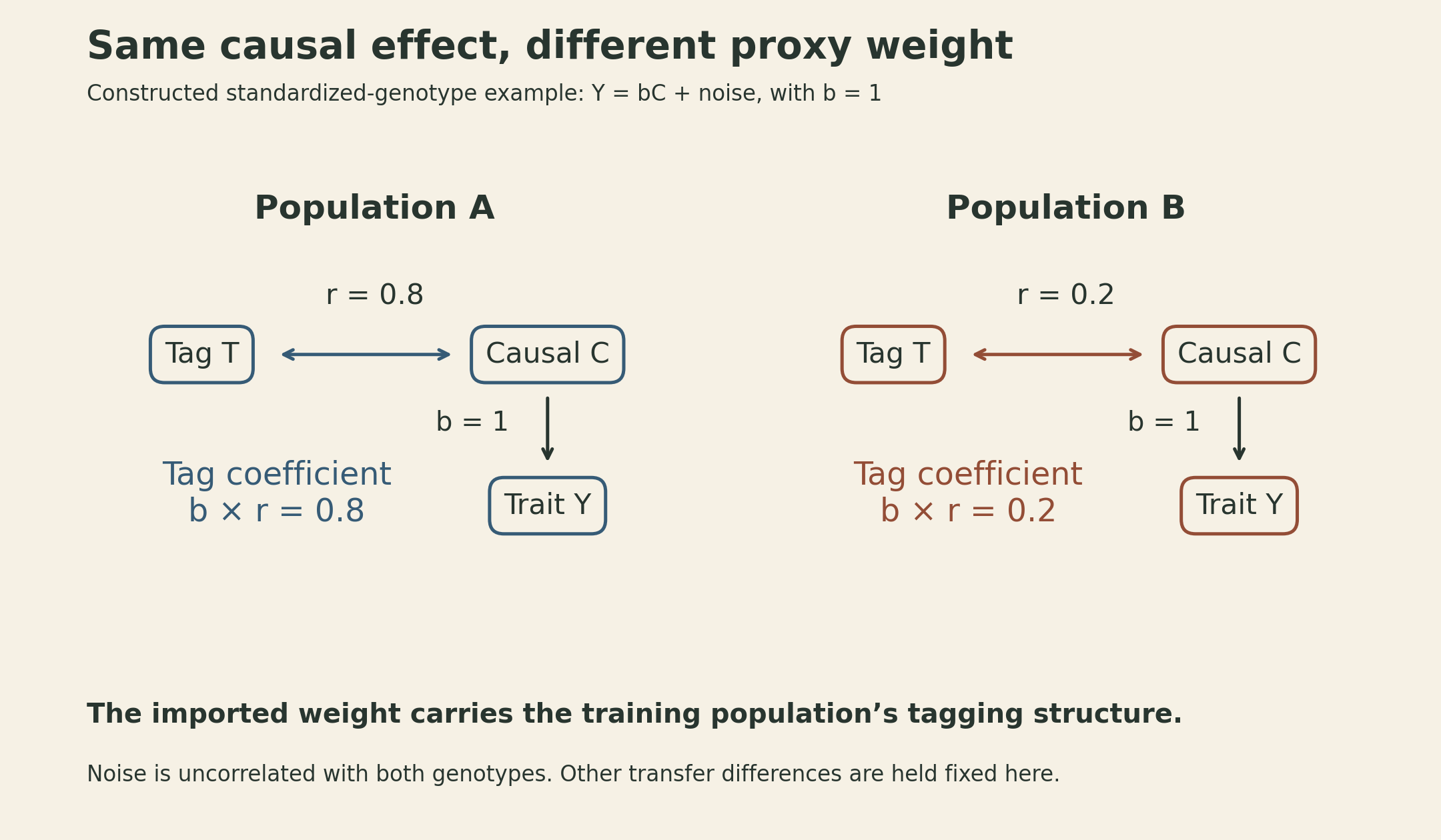
Why can transfer fail even if the underlying causal effect is unchanged? Consider a standardized causal genotype \(C\) and standardized tag \(T\). In a simplified model \(Y=bC+\epsilon\), with noise uncorrelated with both genotypes, the marginal coefficient of the tag is
\[ \frac{\operatorname{Cov}(T,Y)}{\operatorname{Var}(T)} =b\operatorname{Corr}(T,C). \]
If the correlation is 0.8 in one population and 0.2 in another, and \(b=1\), the respective tag coefficients are 0.8 and 0.2. Importing the first coefficient does not import the correlation structure that made it useful. This example holds causal effect and genotype standardization fixed to isolate one failure mode; real transfer differences can also involve allele frequencies, phenotype measurement, environments, and training sample size.
The lecture’s biomarker results show that portability varies by trait, rather than following one universal reduction factor. The reported groupings describe the analyzed test samples; performance still needs to be measured in the intended target population.
The practical distinction at the end of this lecture is between three outputs: an enrichment estimate that prioritizes a biological context, a component that organizes many associations, and a score evaluated for prediction. Each can be valuable. None should be interpreted as one of the others without the additional evidence that interpretation requires.
Lecture and further reading
- MIT 6.874 Spring 2021 course and Lecture 14 materials.
- Systems Genetics lecture slides: mixed models, polygenic scores, heritability, and LD Score regression. The later slides also survey network and sequence-based variant prioritization; those methods complement rather than replace the population-level models here.
- Bulik-Sullivan et al. (2015), LD Score regression.
- Finucane et al. (2015), stratified LD Score regression.
- Tanigawa et al. (2019), DeGAs across 2,138 phenotypes.
- Qian et al. (2020), large-scale sparse regression and snpnet.