Pretraining Fits the Distribution You Choose
CMU Advanced NLP · Lecture 6: Pretraining
A language model can become better at predicting its training text while remaining poor at the task we care about. The gap begins before the optimizer runs: which text entered the corpus, which positions became prediction targets, and how the available computation was divided between parameters and training tokens.
CMU Advanced NLP Lecture 6, taught by Sean Welleck in Fall 2025, connects these choices. Pretraining produces a base model that can be used through prompting or further training. It does not, by itself, specify an assistant’s behavior or guarantee the truth of a continuation.
The useful question is therefore precise: what distribution does the objective reward the model for predicting?
The objective determines what the model can see
Let a token sequence be \(x=(x_1,\ldots,x_T)\). An autoregressive model defines a sequence probability through the chain rule:
\[ p_\theta(x)=\prod_{t=1}^{T}p_\theta(x_t\mid x_{<t}). \]
The empty prefix can be represented by a beginning-of-sequence token; a terminating token is included when modeling variable-length sequences. During training, the target at position \(t\) is the observed \(x_t\), and the input context contains its predecessors. A causal attention mask enforces that information boundary even when many positions are processed in parallel.
Let \(m_{x,t}\in\{0,1\}\) mark whether target \(t\) in sequence \(x\) contributes to the loss, and let \(D_{\mathrm{loss}}=\sum_{x,t}m_{x,t}>0\). A token-averaged negative log likelihood is
\[ \widehat L_{\mathrm{AR}}(\theta) =-\frac{1}{D_{\mathrm{loss}}}\sum_{x\in\mathcal D}\sum_{t=1}^{T_x}m_{x,t} \log p_\theta(x_t\mid x_{<t}). \]
Here \(T_x\) is sequence length, while \(D_{\mathrm{loss}}\) counts only included targets. Padding and any excluded targets have mask zero in both numerator and denominator. This convention matters: averaging the mean token losses equally across documents instead would give tokens in shorter documents more weight.
Masked language modeling asks a different question. Choose a set of target positions \(M\), corrupt the input into \(\widetilde x\), and predict the original tokens at those positions:
\[ L_{\mathrm{MLM}}(\theta) =-\mathbb E_{x,M,\widetilde x} \left[\sum_{i\in M}\log p_\theta(x_i\mid\widetilde x)\right]. \]
The model may use surviving context on both sides. The sum above omits a normalization factor for clarity; practical losses commonly average over selected targets. It is a denoising objective over selected positions, rather than the autoregressive product of prefix-conditioned probabilities.
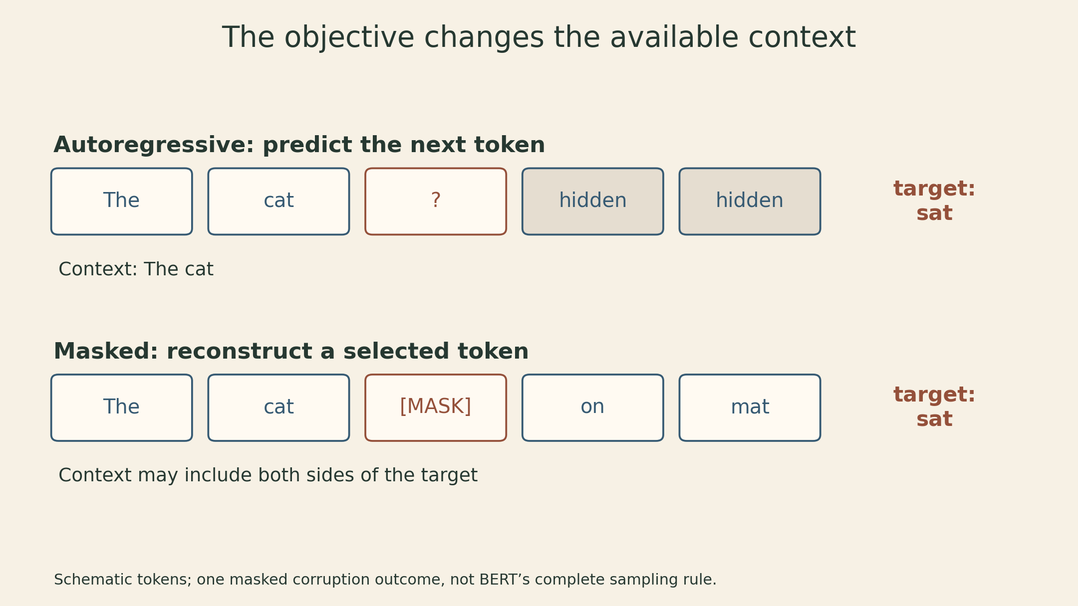
In the original BERT procedure, 15% of WordPiece positions are selected. Within that selected set, 80% are replaced by [MASK], 10% by a random token, and 10% retain the original token. Thus the expected fractions of all positions assigned to those three branches are 12%, 1.5%, and 1.5%. Selection for the loss is distinct from visible replacement. Original BERT also uses next-sentence prediction; MLM alone is not its entire training recipe. BERT, §3.1
The lecture calls MLM a pseudo-likelihood objective. The distinction is that ordinary pseudo-likelihood conditions each variable on all the others, while BERT’s random corruption can hide or alter several positions at once. Neither expression should be substituted for a normalized autoregressive sequence likelihood when comparing objectives.
Maximum likelihood is distribution fitting
Consider a discrete random outcome \(z\) with data distribution \(p_*(z)\) and model distribution \(q_\theta(z)\). It could be a complete sequence or a next token at a fixed context. Assume \(q_\theta(z)>0\) wherever \(p_*(z)>0\). Then
\[ \begin{aligned} \mathrm{KL}(p_*\Vert q_\theta) &=\sum_z p_*(z)\log\frac{p_*(z)}{q_\theta(z)}\\ &=-H(p_*)-\mathbb E_{p_*}[\log q_\theta(z)]. \end{aligned} \]
Equivalently,
\[ H(p_*,q_\theta)=H(p_*)+\mathrm{KL}(p_*\Vert q_\theta). \]
The entropy term does not depend on the model parameters. Minimizing expected negative log likelihood therefore minimizes this forward KL divergence. A finite training average estimates that expectation; it does not reveal the population distribution exactly or guarantee generalization. For token-averaged training, the relevant population includes the context and token weighting induced by the data pipeline.
This also explains the compression connection. With base-2 logarithms, cross entropy is the ideal expected coding cost in bits under the model, up to coding overhead. Natural logarithms give nats; divide by \(\ln 2\) to obtain bits. The expectation is over the data distribution, not samples drawn from the model. Lecture slides, pp. 15–16
A two-outcome example
Suppose, as a constructed example, the true frequencies are \(p_*(A)=0.75\) and \(p_*(B)=0.25\). A model assigning \(q(A)=q(B)=0.5\) has
\[ H_2(p_*,q)=-0.75\log_2 0.5-0.25\log_2 0.5=1\text{ bit}. \]
The data entropy is
\[ H_2(p_*)=-0.75\log_2 0.75-0.25\log_2 0.25\approx0.811278. \]
The mismatch costs about \(0.188722\) extra bits per outcome. Matching the frequencies removes that excess in this idealized example. It says nothing about whether an outcome is desirable or a sentence is factual: the objective rewards probability assigned to observed data.
Even a loss comparison needs a common unit. “Nats per token” from two different tokenizers is not automatically comparable. Held-out text, tokenizer, context length, document boundaries, and loss masking all affect the number being reported.
Filtering changes the distribution, not just the size
A corpus pipeline extracts content, rejects some records, and reduces duplicates. Extraction decides whether equations, code, and paragraph structure survive. Filtering changes which kinds of text are retained. Deduplication changes how much repeated material contributes to training.
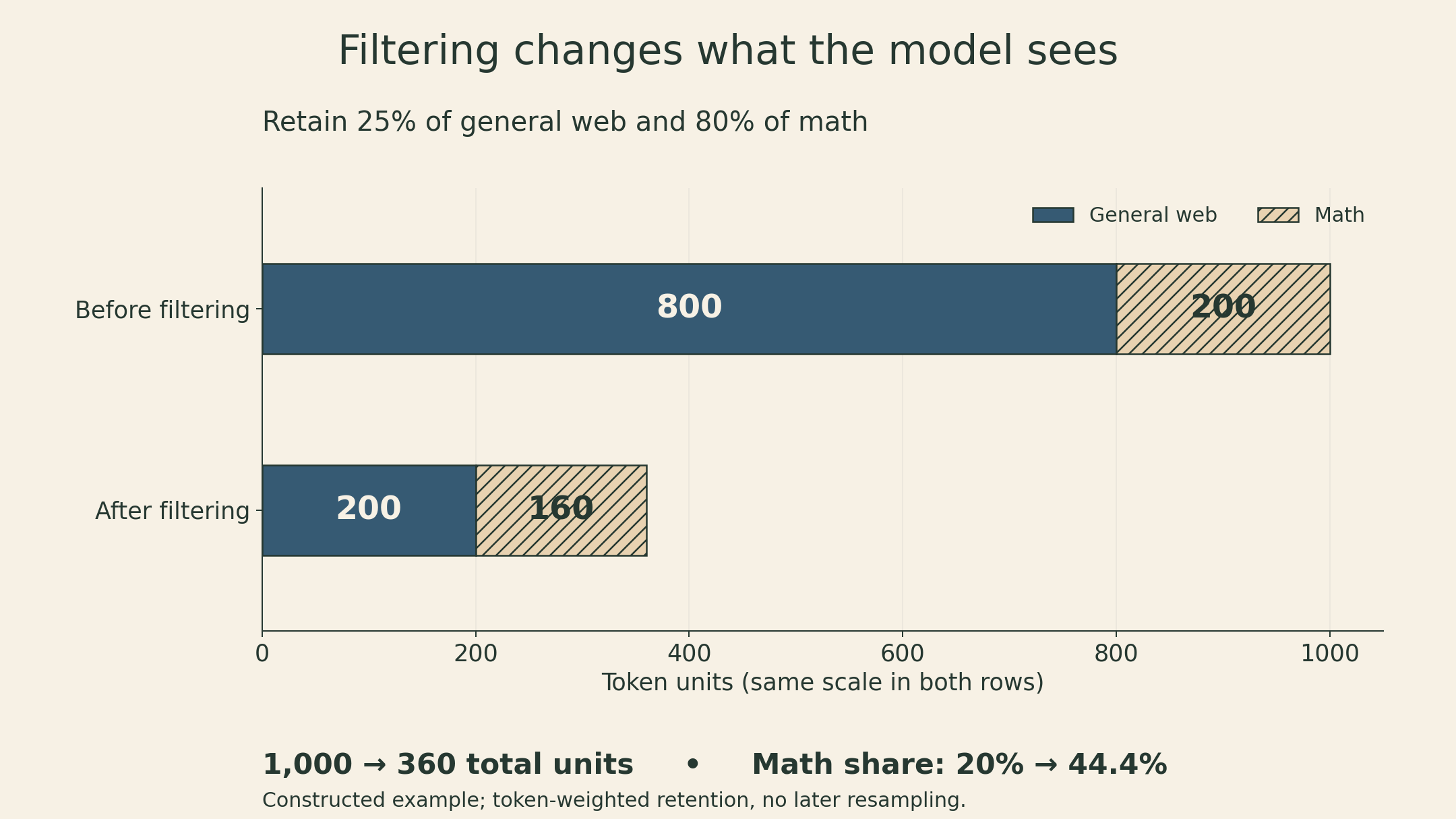
The arithmetic makes this visible. Suppose the initial token mixture has source proportions \(w_k\), and processing retains fraction \(r_k\) of the tokens from source \(k\). With no later resampling, the retained mixture is
\[ w'_k=\frac{w_k r_k}{\sum_j w_j r_j}. \]
Here the retention rates are token-weighted, not merely fractions of documents. Otherwise different document lengths would invalidate the calculation.
Take a constructed corpus of 1,000 token units: 800 general-web units and 200 math units. Keep 25% of the former and 80% of the latter. The result contains 200 general-web units and 160 math units. Math’s share rises from 20% to
\[ \frac{160}{200+160}=\frac49\approx44.4\%. \]
No new math content was added. Its share more than doubled even though math tokens fell from 200 to 160, because general-web text was removed at a much higher rate. A later sampling mixture can change the weights again, and repeated sampling can make training-token count exceed the number of distinct retained tokens.
Classifier filtering puts a learned decision into this pipeline. A classifier trained to recognize mathematical or educational content favors those properties; its score is not a universal measure of usefulness. In FineWeb’s experiments, per-crawl MinHash deduplication outperformed the particular iterative global strategy they tested. That result depends on the deduplication scope and on which documents survived, not simply on removing a larger fraction of text. FineWeb, §3.4
FineWeb-Edu illustrates the separate role of a target criterion: model-generated educational ratings trained a classifier used to select text. The paper’s v2 reports a 1.3T-token subset of 15T-token FineWeb, with gains on its educational benchmark suite. These are results for that selection and evaluation setup, not proof that the same subset is best for every domain. FineWeb, §4
Coverage is consequently an optimization choice. A filter that discards an uncommon format can reduce its weight even if the surviving corpus looks cleaner. Conversely, retaining every format consumes a limited token budget. Evaluating only an overall average can hide the tradeoff.
Compute couples model size to token exposure
For a dense Transformer, a common first-order training estimate is
\[ C\approx6ND, \]
where \(N\) is the parameter count, \(D\) is the number of processed training tokens (including repeated exposures), and \(C\) is floating-point operations. The factor approximates forward and backward arithmetic dominated by parameter matrix multiplications. Attention’s sequence-length-dependent work, activation recomputation, and implementation overhead can change actual cost. FLOPs are not elapsed time, memory use, or a cloud bill. Lecture slides, pp. 47–48
For a rounded 7B-parameter model trained on 2T tokens,
\[ C\approx6(7\times10^9)(2\times10^{12})=8.4\times10^{22}\text{ FLOPs}. \]
The 2T token count is the one reported for Llama 2 pretraining. This arithmetic is an estimate using rounded size, not a reconstruction of its measured hardware cost. Llama 2, §2.1 and Table 1
At that approximate budget, 3.5B parameters with 4T tokens, 7B with 2T, and 14B with 1T all have the same product \(ND\). Equal estimated arithmetic does not imply equal loss or equal runtime. A larger model must learn from fewer token exposures if the budget stays fixed.
What an empirical scaling fit actually decides
The Chinchilla analysis models loss with a fitted expression of the form
\[ \widehat L(N,D)=E+A N^{-\alpha}+B D^{-\beta}, \]
with positive coefficients and exponents. It is a model of measured training outcomes within a setup, not an identity. Its terms represent a fitted floor and finite-model/data contributions. The study’s methods favored roughly balanced growth of parameters and tokens as compute increased. Hoffmann et al., §3
The tradeoff can be derived without borrowing any fitted coefficients. Substitute \(D=C/(6N)\) and differentiate with respect to \(\log N\) at fixed \(C\):
\[ \left.\frac{d\widehat L}{d\log N}\right|_C =-\alpha A N^{-\alpha}+\beta B D^{-\beta}. \]
At an interior optimum,
\[ \alpha A N^{-\alpha}=\beta B D^{-\beta}. \]
The marginal benefit of more parameters balances the cost of fewer tokens. In this fitted family,
\[ N_{\mathrm{opt}}\propto C^{\beta/(\alpha+\beta)}, \qquad D_{\mathrm{opt}}\propto C^{\alpha/(\alpha+\beta)}. \]
Equal exponents yield square-root growth of both quantities. They do not imply a universal optimal tokens-per-parameter ratio.
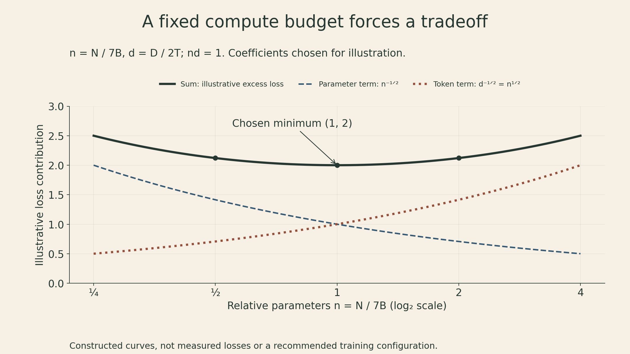
The figure deliberately uses a constructed symmetric function. Define \(n=N/(7\mathrm B)\) and \(d=D/(2\mathrm T)\), so \(nd=1\) at the example budget. Set
\[ \ell(n,d)=n^{-1/2}+d^{-1/2}=n^{-1/2}+n^{1/2}. \]
It reaches 2 at \(n=1\) and about 2.121 at both \(n=0.5\) and \(n=2\). This demonstrates the balance, not an empirical recommendation to train a 7B model on 2T tokens. Changing either coefficient moves the minimum.
Scaling studies also use smaller runs to investigate learning rates and batch sizes. Their extrapolations inherit the data, architecture, optimizer, and measurement conditions of those runs. A power-law exponent drawn on a lecture plot is not a constant to apply to every future training job. Training-compute optimality also leaves out the number and cost of future inference requests.
The notebook demonstrates a base model, not a training run
The lecture notebook at commit 8f5328f loads HuggingFaceTB/SmolLM2-360M with AutoModelForCausalLM. It tokenizes prompts, calls generate, and decodes the result. There is no optimizer or pretraining loop in this demonstration.
The prompts include an arithmetic expression and a factual-completion prompt about past weather in Pittsburgh. A plausible continuation is not evidence that arithmetic is reliable or that the weather is correct. That would require task-specific ground truth and an evaluation protocol. The base checkpoint is also distinct from an instruction-tuned variant.
Two implementation details affect what can be reproduced. The notebook upgrades transformers without fixing a version and loads the model without a revision pin. Its generate call does not explicitly set sampling or output length, so those behaviors depend on the loaded configuration and library version; the printed decode also includes the input prompt.
The Dolma example downloads cc_en_head-0000.json.gz, then asks head to read cc_en_head-0000.json. The displayed cells omit decompression. With only the downloaded compressed file present, the latter path is missing. A direct way to read one JSONL record from the compressed file is:
import gzip
import json

with gzip.open("cc_en_head-0000.json.gz", "rt", encoding="utf-8") as f:
    record = json.loads(next(f))
print(record.keys())
This assumes the referenced gzip file has already been downloaded and contains a JSON object on each line. It only illustrates record access; it does not implement extraction, filtering, deduplication, or pretraining.
The loss only answers its own question
For a held-out loss to be useful, the held-out distribution and scoring convention must be clear. For downstream evaluation, prompt format, demonstrations, decoding, and any fine-tuning become part of the experiment. Lower training loss, lower held-out loss, and better downstream performance are related observations, not interchangeable claims.
The connection across this lecture is concrete. The objective chooses the prediction problem. The data pipeline determines the examples and their weights. The compute budget limits how much model capacity and token exposure can be purchased together. Interpreting a pretrained model requires all three—not just its parameter count.
Sources
- Sean Welleck, CMU Advanced NLP Fall 2025, Lecture 6: Pretraining, September 11, 2025; slides adapted from Graham Neubig’s Fall 2024 course; course schedule.
- Lecture notebook, fixed commit
8f5328f. - Devlin et al., BERT, §3.1.
- Penedo et al., The FineWeb Datasets, §§3.4 and 4.
- Touvron et al., Llama 2, §2.1 and Table 1.
- Hoffmann et al., Training Compute-Optimal Large Language Models, §3.